Gray Correlation for Vertical Two-Phase Flow: Engineering Fundamentals
Calculate bottomhole pressure, predict liquid holdup, and analyze gas well performance using Gray's dimensionless number approach. Industry-standard method for high-GLR gas wells per API 14B.
Calculate bottomhole pressure from wellhead conditions
Predict liquid loading onset in gas wells
Size tubing for gas well completions
Evaluate gas lift requirements
1. Overview & Applications
The Gray correlation (1974) is an empirical method for calculating pressure drop in vertical two-phase gas-liquid flow. Developed by H.E. Gray for the API 14B standard on subsurface safety valve sizing, it uses dimensionless groups to correlate liquid holdup with flow conditions.
Primary Use
BHP from Wellhead
Calculate bottomhole flowing pressure given wellhead pressure, flow rates, and fluid properties.
Liquid Loading
Critical Velocity
Determine if gas velocity is sufficient to lift liquids from wellbore (Turner criteria).
Tubing Design
Size Optimization
Balance pressure drop vs. liquid lifting capacity when selecting tubing size.
Gas Lift
Injection Rate
Calculate required gas injection to achieve target bottomhole pressure.
Key Concepts
Two-phase flow: Simultaneous flow of gas and liquid in a conduit; behavior differs from single-phase due to phase interactions
Liquid holdup (HL): Fraction of pipe cross-section occupied by liquid; determines mixture density
Slippage: Gas travels faster than liquid due to buoyancy; causes liquid to accumulate
No-slip holdup (λ): Input liquid fraction if phases traveled at same velocity; λ = Ql/(Ql+Qg)
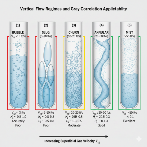
Vertical flow regime progression with Gray correlation applicability ratings for each pattern.
Flow Regime Applicability
Flow Regime
Vsg Range
Characteristics
Gray Accuracy
Bubble
< 3 ft/s
Discrete gas bubbles in liquid
Poor (not designed for this)
Slug
3-10 ft/s
Alternating liquid slugs/gas pockets
Moderate (±20-30%)
Churn
10-20 ft/s
Chaotic oscillating flow
Moderate (±15-25%)
Annular
20-50 ft/s
Liquid film on wall, gas core
Good (±10-15%)
Mist
> 50 ft/s
Liquid droplets in gas
Excellent (±5-10%)
Gray is a single continuous correlation: unlike Duns-Ros, Gray does not switch equations by flow regime. The regimes above are shown only as a qualitative guide to where Gray is most reliable. The flow-pattern label in the calculator is an informational Duns-Ros-style add-on, not part of the Gray pressure-traverse math.
When to use Gray: Vertical or near-vertical wells (<15° deviation) with high GLR (>5,000 scf/bbl) operating in annular or mist flow. For oil wells or high liquid loading, use Hagedorn-Brown instead.
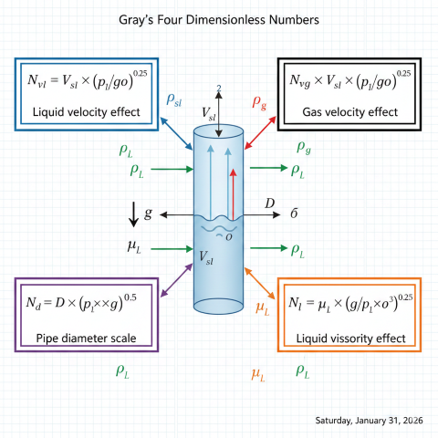
2. Gray Dimensionless Numbers
Gray's correlation uses two dimensionless groups built from the no-slip mixture density, the mixture superficial velocity, the density difference and surface tension. The leading constant 453.592 absorbs the unit conversion so that surface tension is supplied directly in dyne/cm. Note that Nv uses the mixture velocity raised to the fourth power.
No-Slip Mixture Density (ρns):
ρns = ρL × λL + ρg × (1 − λL)
where λL = Vsl / (Vsl + Vsg) (no-slip liquid holdup)
and Vm = Vsl + Vsg (mixture superficial velocity)
Gray Velocity Number (Nv):
Nv = 453.592 × ρns² × Vm⁴ / (gc × σ × (ρL − ρg))
Where:
ρns = No-slip mixture density (lbm/ft³)
Vm = Mixture superficial velocity (ft/s) — note the 4th power
gc = 32.17 lbm·ft/(lbf·s²)
σ = Surface tension (dyne/cm, used directly)
Gray Pipe Diameter Number (Nd):
Nd = 453.592 × gc × (ρL − ρg) × D² / σ
Where:
D = Pipe inside diameter (ft)
σ = Surface tension (dyne/cm)
Physical Interpretation
Number
Physical Meaning
Typical Range (gas wells)
Nv
Mixture-inertia to surface-tension / buoyancy forces (Vm⁴ dependence)
10² - 10⁶
Nd
Buoyancy (gravitational) to surface-tension forces at pipe scale
500 - 5,000
Gray dimensionless numbers showing how physical variables combine into correlating parameters.
Gray's liquid holdup is a single closed-form expression in the dimensionless numbers Nv and Nd and the superficial velocity ratio R. There is no flow-regime switching and no iterative chart lookup — the gas void fraction fg falls out directly, and the in-situ liquid holdup is HL = 1 − fg. The result is always at least the no-slip holdup, because gas slips past the slower liquid.
No-Slip Liquid Holdup:
λL = Vsl / (Vsl + Vsg) = Ql / (Ql + Qg)
This is the holdup if both phases traveled at the same velocity.
Superficial Velocity Ratio:
R = Vsl / VsgGray B coefficient:
B = 0.0814 × (1 − 0.0554 × ln(1 + 730·R/(R + 1)))
Gray A exponent:
A = −2.314 × ( Nv × (1 + 205/Nd) )BGas Void Fraction and Liquid Holdup:
fg = (1 − eA) / (R + 1)
HL = 1 − fg (clamped to λL ≤ HL ≤ 1)
Slip Ratio:
S = HL / λL (typically ~1.2-3× in high-GLR mist/annular wells; larger at lower gas velocity)
Worked Example (mid-well, from Section 2):
Nv = 1.84×10⁵, Nd = 1,338, R = 0.10/36.5 = 0.00274
B = 0.0814 × (1 − 0.0554 × ln(1 + 730×0.00274/1.00274)) = 0.0765
A = −2.314 × (1.84×10⁵ × (1 + 205/1338))0.0765 = −5.91
fg = (1 − e−5.91) / 1.00274 = 0.995
HL = 1 − 0.995 = 0.0054 (≈ 0.54% — vs no-slip λL = 0.27%, an ~2× slip ratio)
Effect of Holdup on Pressure Drop
Liquid holdup directly affects mixture density, which dominates pressure gradient in vertical wells:
Slip (in-situ) Mixture Density — used for hydrostatic head:
ρs = ρL × HL + ρg × (1 − HL)
Example:
If ρL = 46.7 lbm/ft³, ρg = 2.42 lbm/ft³, HL = 0.0054:
ρs = 46.7 × 0.0054 + 2.42 × 0.9946 = 0.25 + 2.41 = 2.66 lbm/ft³
Compare to no-slip (λL = 0.00273):
ρns = 46.7 × 0.00273 + 2.42 × 0.997 = 2.54 lbm/ft³
Error = (2.66 − 2.54)/2.66 ≈ 5% in this high-velocity mist case (slip ≈ 2×).
At lower gas velocity slip — and the head error from ignoring it — grow quickly
(see the sensitivity table below), which is why Gray solves for HL rather than assuming no-slip.
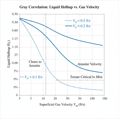
Holdup Sensitivity Table
Vsg (ft/s)
Vsl (ft/s)
λ (%)
HL (%)
Slip Ratio
Flow Regime
10
0.1
0.99
2.94
3.0×
Churn
25
0.1
0.40
0.94
2.4×
Annular
50
0.1
0.20
0.34
1.7×
Mist
25
0.5
1.96
2.58
1.3×
Annular
50
0.5
0.99
1.18
1.2×
Mist
Gray correlation liquid holdup as a function of gas velocity for different liquid loading conditions.
4. Pressure Gradient Calculation
Total pressure gradient in vertical two-phase flow has three components: elevation (hydrostatic head), friction, and acceleration. For most gas well conditions, elevation dominates (80-95% of total).
Total Pressure Gradient:
(dP/dL)total = (dP/dL)elevation + (dP/dL)friction + (dP/dL)accelerationElevation Component (dominant in vertical flow) — uses SLIP density:
(dP/dL)elev = ρs × (g/gc) × cos(θ) / 144 [psi/ft]
Where:
ρs = Slip (in-situ) mixture density = ρL·HL + ρg·(1 − HL)
g/gc = 1.0 (gravitational constant ratio, dimensionless in lbm/lbf system)
θ = Deviation from vertical (degrees)
144 = Conversion factor (in²/ft²)
Friction Component — uses NO-SLIP density and Gray's pseudo roughness:
(dP/dL)fric = f × ρns × Vm² / (2 × gc × D × 144) [psi/ft]
Where:
f = Darcy friction factor from Colebrook/Jain, evaluated with the
Gray effective relative roughness ε/D = ke/D (NOT bare pipe roughness):
ke = (28.5/453.592) × σ / (ρns × Vm²) for R = Vsl/Vsg ≥ 0.007
(blended toward the bare wall roughness ε for R < 0.007; floor ke ≥ 2.77×10⁻⁵ ft)
ρns = No-slip mixture density (lbm/ft³)
Vm = Vsl + Vsg (mixture velocity, ft/s)
gc = 32.17 lbm·ft/(lbf·s²), D = Pipe ID (ft)
Acceleration Component:
Usually negligible for steady-state vertical flow (< 1% of total)
Bottomhole Pressure Calculation
For vertical well (θ = 0°):
PBH = PWH + ∫ (dP/dL)total dL (marched surface → bottom)
Example Calculation (multi-segment march):
Given: PWH = 500 psia, TVD = 8,000 ft, D = 0.2034 ft
The calculator integrates the Gray gradient in 60 depth steps, updating
Z, ρg, Vsg, holdup and friction at the local P,T of each step.
At the representative mid-well point (P ≈ 755 psia, T ≈ 132°F):
ρs = 4.15 lbm/ft³, ρns = 2.54 lbm/ft³
Vm = 36.6 ft/s, f ≈ 0.019 (with ke ≈ 1.75×10⁻⁴ ft, ε/D ≈ 8.6×10⁻⁴)
Elevation gradient (slip density, g/gc = 1.0):
(dP/dL)elev = 4.15 / 144 = 0.0289 psi/ft
Friction gradient (no-slip density, pseudo roughness):
(dP/dL)fric = 0.019 × 2.54 × 36.6² / (2 × 32.17 × 0.2034 × 144)
(dP/dL)fric ≈ 0.0345 psi/ft
Mid-well total gradient ≈ 0.063 psi/ft. Integrating the full traverse
(gradient rises with depth as pressure and holdup increase) gives:
Bottomhole pressure:
PBH ≈ 1,010 psia (total ΔP ≈ 510 psi over 8,000 ft)
Note: A single-segment calculation seeded at an over-high
average pressure inflates both holdup and BHP (the legacy engine returned
~1,572 psia). Marching from surface to bottom with property updates at
each step is self-consistent and lands BHP in the defensible
≈ 950-1,100 psia range for these conditions.
Turner Critical Velocity
The minimum gas velocity to prevent liquid accumulation (loading) in vertical wells:
Gray is one of several empirical correlations for vertical two-phase flow. Selection depends on well type, flow regime, and accuracy requirements.
Correlation Comparison Table
Correlation
Year
Best Application
Limitations
Gray
1974
High GLR gas wells, mist/annular flow
Poor for slug flow, liquid loading
Hagedorn-Brown
1965
Oil wells, high liquid loading, slug flow
Complex charts, less accurate for gas wells
Beggs-Brill
1973
Inclined/horizontal flow, all angles
Developed for horizontal; less accurate for vertical
Duns-Ros
1963
Wide range, flow regime maps
Discontinuities at transitions, complex
Ansari (mechanistic)
1994
All conditions, physics-based
Computationally intensive
When to Use Each Method
Decision Guide:
1. Is it a gas well with GLR > 5,000 scf/bbl?
→ YES: Use Gray (or Duns-Ros)
→ NO: Go to step 2
2. Is liquid loading a concern (low gas rate)?
→ YES: Use Hagedorn-Brown or Ansari mechanistic
→ NO: Go to step 3
3. Is deviation > 15° from vertical?
→ YES: Use Beggs-Brill
→ NO: Gray or Hagedorn-Brown acceptable
4. Is high accuracy required (±5%)?
→ YES: Use mechanistic model (Ansari, Hasan-Kabir)
→ NO: Gray is acceptable for screening
Industry Practice:
Run multiple correlations and compare. If results differ by >20%,
investigate flow regime and validate with field pressure surveys.
Accuracy Comparison (Field Studies)
Well Type
Gray Error
Hagedorn-Brown Error
Recommended
High-rate gas (>5 MMscfd)
±8%
±15%
Gray
Low-rate gas with loading
±25%
±12%
Hagedorn-Brown
Gas condensate (20-50 bbl/MMscf)
±12%
±10%
Either acceptable
Oil well (GOR > 1,000)
±18%
±9%
Hagedorn-Brown
Summary: Gray correlation is the industry standard for vertical gas wells with high GLR operating in annular or mist flow. For oil wells, high liquid loading, or slug flow conditions, Hagedorn-Brown provides better accuracy. Always validate predictions with measured bottomhole pressure when available.
When should the Gray correlation be used instead of other multiphase flow methods?+
The Gray correlation is specifically designed for high gas-liquid ratio (GLR > 5,000 scf/bbl) vertical flow in gas wells. It achieves ±10–15% accuracy for gas-condensate wells and is preferred over Hagedorn-Brown for very high GLR applications.
What are the key dimensionless numbers used in the Gray correlation?+
The Gray correlation uses dimensionless numbers based on liquid velocity, gas velocity, pipe diameter, and surface tension to characterize two-phase flow behavior. These numbers are combined in Gray's closed-form expression (coefficients B and A) to determine the gas void fraction and the in-situ liquid holdup.
What is the primary application of the Gray vertical flow correlation?+
The Gray correlation is primarily used for calculating bottomhole pressure from wellhead measurements in gas wells, sizing production tubing, determining critical velocity for liquid unloading, and calculating injection rates for gas lift design.