The industry-standard empirical method for calculating pressure gradients in vertical gas wells. Predicts liquid holdup and bottom-hole pressure using dimensionless groups derived from extensive field data.
The Hagedorn-Brown correlation, published in JPT April 1965 (SPE-940-PA), remains one of the most widely used methods for vertical multiphase flow calculations. It provides a unified approach that handles all flow regimes without discontinuities at regime transitions.
Development Background
A.R. Hagedorn and K.E. Brown developed this correlation at the University of Tulsa using:
1,500-ft test well with 1.0", 1.25", and 1.5" tubing
475 pressure traverse measurements across various flow conditions
Back-calculated holdup values from measured pressure drops
Dimensionless groups adapted from Duns and Ros (1963)
Key insight: Unlike flow-regime-specific methods (Duns-Ros, Orkiszewski), Hagedorn-Brown uses a single continuous correlation for all flow patterns, avoiding discontinuities that can cause numerical instabilities in iterative calculations.
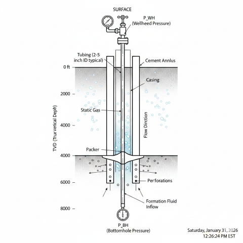
Vertical well schematic showing tubing, casing, and pressure measurement points for traverse analysis.
Application Range
Parameter
Original Data Range
Recommended Limits
Tubing ID
1.0" - 1.5"
1.0" - 4.0"
Liquid Rate
0 - 2,000 bbl/d
0 - 10,000 bbl/d
GLR
50 - 3,000 scf/bbl
50 - 50,000 scf/bbl
Deviation
Vertical only
< 15° from vertical
Oil Viscosity
0.5 - 110 cP
0.1 - 200 cP
2. Dimensionless Numbers
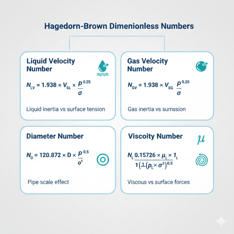
The correlation uses four dimensionless groups that characterize the flow conditions. These numbers relate fluid properties, flow velocities, and pipe geometry in a way that allows correlation of experimental data.
Liquid Velocity Number (NLV)
Definition:
NLV = 1.938 × vSL × (ρL / σ)0.25
Where:
vSL = Superficial liquid velocity (ft/s)
ρL = Liquid density (lb/ft³)
σ = Liquid-gas surface tension (dyne/cm)
1.938 = Unit conversion factor for field units
Gas Velocity Number (NGV)
Definition:
NGV = 1.938 × vSG × (ρL / σ)0.25
Where:
vSG = Superficial gas velocity at flowing conditions (ft/s)
Note: Gas velocity must be calculated at actual P and T:
vSG = Qg,std × (Pb/P) × (T/Tb) × Z / (86400 × A)
Where Pb = 14.7 psia, Tb = 520°R (standard conditions)
Pipe Diameter Number (ND)
Definition:
ND = 120.872 × D × (ρL / σ)0.5
Where:
D = Tubing inside diameter (ft)
120.872 = Unit conversion factor for field units
Liquid Viscosity Number (NL)
Definition:
NL = 0.15726 × μL × (1 / (ρL × σ³))0.25
Where:
μL = Liquid viscosity (cP)
0.15726 = Unit conversion factor for field units
Hagedorn-Brown dimensionless groups showing physical interpretation of each parameter.
Typical Values
Number
Low GLR Oil Well
Gas-Condensate Well
High-Rate Gas Well
NLV
5 - 50
0.5 - 5
0.01 - 0.5
NGV
10 - 100
50 - 500
200 - 2000
ND
20 - 200 (geometry dependent)
NL
0.001 - 0.1
0.0001 - 0.01
0.0001 - 0.001
3. Liquid Holdup Correlation
Liquid holdup (HL) is the fraction of the pipe cross-section occupied by liquid at any instant. It differs from the input liquid fraction (λL) because gas flows faster than liquid—this velocity difference is called "slip."
Holdup vs. No-Slip Holdup
No-slip (input) liquid fraction:
λL = vSL / (vSL + vSG) = vSL / vmActual liquid holdup:
HL ≥ λL (always, due to slip)
Physical meaning:
• λL = 0.05 means 5% of inlet flow is liquid
• HL = 0.20 means 20% of pipe volume is liquid
• Difference indicates liquid accumulation due to slower liquid velocity
Hagedorn-Brown Holdup Procedure
The correlation uses three steps with polynomial curve fits:
Step 1: Calculate CNL from NL
Viscosity correction factor:
CNL = 0.061 × NL³ - 0.0929 × NL² + 0.0505 × NL + 0.0019
This polynomial fits the original H-B Figure 3 correlation chart.
Step 2: Calculate correlation groups H and B
Primary correlating group (H):
H = (NLV / NGV0.575) × (P / 14.7)0.1 × CNL / NDSecondary correlating group (B):
B = (NGV × NLV0.38) / ND2.14
Step 3: Calculate ψ factor and HL
ψ factor (piecewise polynomial):
If B ≤ 0.025:
ψ = 27170×B³ - 317.52×B² + 0.5472×B + 0.9999
If 0.025 < B ≤ 0.055:
ψ = -533.33×B² + 58.524×B + 0.1171
If B > 0.055:
ψ = 2.5714×B + 1.5962
Holdup ratio from H group:
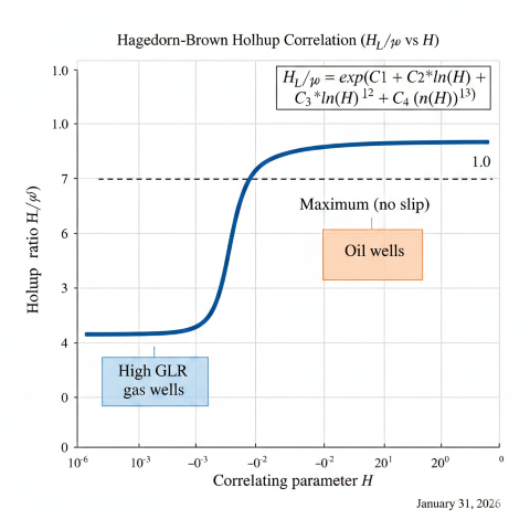
HL/ψ = √[(0.0047 + 1123.32×H + 729489.64×H²) / (1 + 1097.1566×H + 722153.97×H²)]
Final liquid holdup:
HL = (HL/ψ) × ψ
Constraint: HL ≥ λL (physical requirement)
Hagedorn-Brown holdup correlation relating HL/ψ to the correlating parameter H.
Griffith Bubble Flow Modification
For bubble flow regime, the original H-B method can underpredict holdup. A modification using the Griffith correlation is applied:
Bubble flow criterion:
LB = max(1.071 - 0.2218 × vm² / D, 0.13)
If λg < LB, use Griffith holdup:
Griffith holdup:
HL = 1 - 0.5 × [1 + vm/vs - √((1 + vm/vs)² - 4×vSG/vs)]
Where vs = 0.8 ft/s (slip velocity for large bubbles)
Holdup and Flow Patterns
Flow Pattern
Typical HL
GLR Range
Characteristics
Bubble
0.70 - 0.95
< 500
Discrete gas bubbles in liquid
Slug
0.40 - 0.70
500 - 2,000
Alternating liquid slugs and gas pockets
Churn/Transition
0.25 - 0.40
2,000 - 5,000
Chaotic, oscillatory flow
Annular/Mist
0.05 - 0.25
> 5,000
Liquid film on wall, gas core with droplets
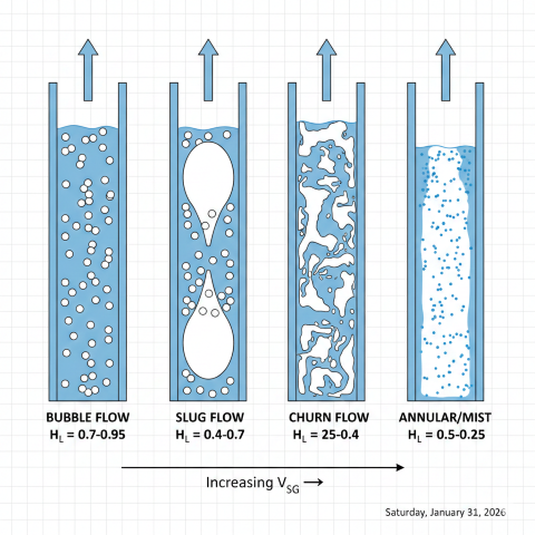
Vertical multiphase flow patterns showing progression from bubble to annular/mist with increasing gas velocity.
4. Pressure Gradient Calculation
The total pressure gradient consists of three components: elevation (hydrostatic), friction, and acceleration. For most gas well applications, acceleration is negligible.
Total Pressure Gradient
General form:
(dP/dL)total = (dP/dL)elevation + (dP/dL)friction + (dP/dL)acceleration
For steady-state gas wells (acceleration ≈ 0):
(dP/dL)total ≈ (dP/dL)h + (dP/dL)f
Units: psi/ft
Elevation (Hydrostatic) Component
Elevation gradient:
(dP/dL)h = ρm / 144
Where mixture density:
ρm = ρL × HL + ρg × (1 - HL)
Units: ρ in lb/ft³, result in psi/ft
For deviated wells:
(dP/dL)h,deviated = (dP/dL)h × cos(θ)
Where θ = deviation angle from vertical
Friction Component
Friction gradient (uses no-slip density per SPE-940-PA):
(dP/dL)f = (f × ρn × vm²) / (2 × gc × D × 144)
Where:
f = Darcy friction factor (from Colebrook-White)
ρn = ρL × λL + ρg × (1 - λL) (no-slip density)
vm = vSL + vSG (mixture velocity, ft/s)
gc = 32.174 lbm·ft/(lbf·s²)
D = Tubing ID (ft)
Note: The elevation component uses slip density ρs = ρL×HL + ρg×(1-HL), but the friction component uses no-slip density ρn. The original H-B correlation was calibrated by back-calculating holdup from measured pressure drops using ρn for the friction term (Brill & Mukherjee, 1999).
Two-phase Reynolds number (no-slip basis):
Re = ρn × vm × D / μnNo-slip viscosity (geometric mean):
μn = μLλL × μg(1-λL)
Colebrook-White Friction Factor
Implicit equation (requires iteration):
1/√f = -2 × log₁₀(ε/(3.7×D) + 2.51/(Re×√f))
Where:
ε = Pipe roughness (0.0006 in for commercial steel tubing)
D = Pipe diameter (in, same units as ε)
Typical friction factors:
Smooth pipe: f = 0.015 - 0.020
Tubing: f = 0.018 - 0.025
Corroded: f = 0.025 - 0.040
Component Comparison
Well Type
Elevation %
Friction %
Dominant Factor
Low-rate oil well
95 - 99%
1 - 5%
Hydrostatic (high HL)
Gas-condensate well
85 - 95%
5 - 15%
Hydrostatic
High-rate gas well
60 - 85%
15 - 40%
Both significant
Very high rate
40 - 60%
40 - 60%
Friction increases
5. Worked Example
Calculate the bottom-hole pressure for a gas well producing through 2.875" (2.441" ID) tubing.
Interpretation: Low liquid holdup (9.2%) indicates the well is in annular/mist flow with efficient liquid removal. The pressure gradient is strongly dominated by the elevation component (92%), which is characteristic of gas wells. Using the no-slip density for friction (per SPE-940-PA calibration basis) gives a lower friction contribution than the slip density approach. No artificial lift is needed at these conditions.
6. Correlation Selection Guide
Multiple multiphase flow correlations exist for different applications. Selection depends on well geometry, flow regime, and required accuracy.
Correlation Comparison
Correlation
Year
Best For
Limitations
Hagedorn-Brown
1965
Vertical gas wells, all flow regimes
Vertical only; empirical
Beggs-Brill
1973
Deviated/horizontal wells
Less accurate for vertical
Duns-Ros
1963
Vertical, regime-specific
Discontinuities at transitions
Orkiszewski
1967
Combines best methods
Complex implementation
Gray
1974
Quick gas well estimates
Lower accuracy
Mechanistic (OLGA)
Modern
Complex systems, transients
Requires software
Selection Flowchart
Decision process:
1. Is well vertical or near-vertical (<15°)?
YES → Use Hagedorn-Brown
NO → Use Beggs-Brill
2. Is it a high-rate gas well?
YES → Hagedorn-Brown is excellent
NO → Continue evaluation
3. Need flow regime identification?
YES → Consider Duns-Ros or Orkiszewski
NO → Hagedorn-Brown (unified approach)
4. Deviated well (15-60°)?
→ Use Beggs-Brill with inclination correction
5. Horizontal well?
→ Use Beggs-Brill or Eaton-Brown
Recommendation:
• Preliminary: Gray correlation (quick estimates)
• Design: Hagedorn-Brown (industry standard)
• Critical: Mechanistic model + field calibration
Accuracy Summary
Application
H-B Accuracy
When to Use Alternative
High-rate vertical gas well
± 10%
Never—this is H-B's strength
Gas-condensate well
± 15%
Only if field data shows bias
Loaded gas well
± 15-20%
Consider Turner criterion also
Oil well (low GOR)
± 20%
Consider Duns-Ros or Orkiszewski
Deviated well (>15°)
Poor
Use Beggs-Brill
Best practice: For critical applications, compare 2-3 correlations and validate against field pressure surveys. Hagedorn-Brown typically provides reliable middle-range predictions for vertical gas wells. When possible, tune the correlation to field data by adjusting holdup predictions.
What is the Hagedorn-Brown correlation and when is it used?+
The Hagedorn-Brown correlation is a vertical multiphase flow method developed from over 1,000 well tests. It predicts liquid holdup and pressure gradient in vertical gas wells and is the industry standard for production tubing design with ±10–15% accuracy.
What dimensionless numbers are used in the Hagedorn-Brown method?+
Four dimensionless numbers characterize the flow: liquid velocity number, gas velocity number, pipe diameter number, and liquid viscosity number. These are calculated from superficial velocities, fluid properties, and pipe geometry to correlate liquid holdup.
How does the Hagedorn-Brown holdup differ from no-slip holdup?+
No-slip holdup assumes both phases travel at the same velocity, while actual holdup accounts for gas slippage past the slower liquid phase. The Hagedorn-Brown correlation uses empirical charts to determine the actual holdup ratio, which is always greater than or equal to no-slip holdup.