1. Correlation Overview
The Beggs-Brill (1973) correlation predicts pressure drop and liquid holdup for two-phase gas-liquid flow in pipes at any inclination angle. It remains widely used for gathering systems and pipelines.
Key Features
Inclination
-90° to +90°
Robust for downhill liquid draining and uphill accumulation scenarios.
Regimes
4 patterns
Segregated, intermittent, distributed, transition via λL and NFR.
Holdup
Inclination-corrected
Starts with horizontal holdup, then applies ψ(θ) factor.
Friction
2Φ multiplier
Single-phase Moody factor with S-based multiplier for slip.
Input Parameters
| Parameter | Symbol | Units |
|---|---|---|
| Superficial gas velocity | V_sg | ft/s |
| Superficial liquid velocity | V_sl | ft/s |
| Pipe inside diameter | D | ft |
| Inclination angle | θ | degrees |
| Gas density | ρ_g | lb/ft³ |
| Liquid density | ρ_l | lb/ft³ |
| Gas viscosity | μ_g | cp |
| Liquid viscosity | μ_l | cp |
| Surface tension | σ | dyne/cm |
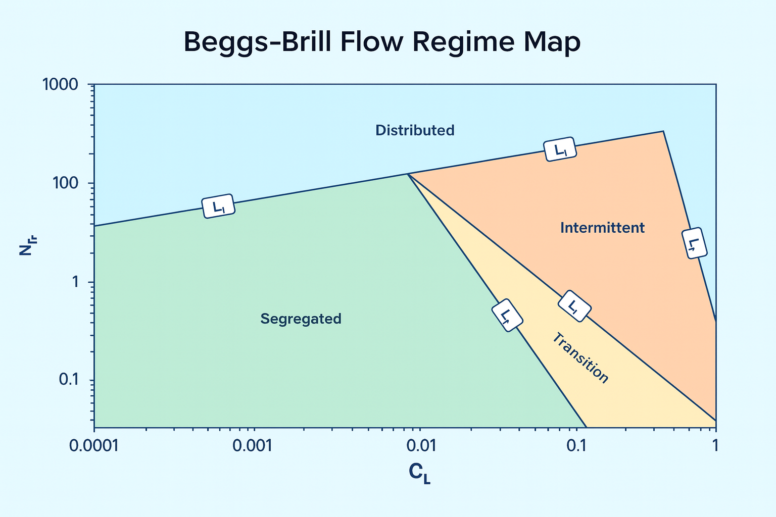
2. Flow Regime Determination
Beggs-Brill identifies four flow patterns based on dimensionless parameters:
Calculate λL and NFR. Use superficial velocities and diameter; keep units consistent.
Pick the regime. Compare NFR to L1–L4; flag if λL is outside test range.
Select coefficients. Regime drives holdup constants and inclination correction factors.
Flow Regime Map
| Regime | Condition | Description |
|---|---|---|
| Segregated | λ_L < 0.01 and N_FR < L1 or λ_L ≥ 0.01 and N_FR < L2 |
Stratified or annular; phases separated |
| Intermittent | 0.01 ≤ λ_L < 0.4 and L3 < N_FR ≤ L1 or λ_L ≥ 0.4 and L3 < N_FR ≤ L4 |
Slug or plug flow; alternating phases |
| Distributed | λ_L < 0.4 and N_FR ≥ L1 or λ_L ≥ 0.4 and N_FR > L4 |
Bubble or mist; phases well-mixed |
| Transition | L2 < N_FR < L3 | Between segregated and intermittent |
3. Liquid Holdup
Liquid holdup (H_L) is the fraction of pipe volume occupied by liquid. Beggs-Brill calculates horizontal holdup first, then corrects for inclination.
Horizontal Holdup (H_L(0))
Inclination Correction
Inclination Coefficients
| Regime | d | e | f | g |
|---|---|---|---|---|
| Segregated uphill | 0.011 | -3.768 | 3.539 | -1.614 |
| Intermittent uphill | 2.96 | 0.305 | -0.4473 | 0.0978 |
| Distributed uphill | No correction (C = 0) | |||
| All regimes downhill | 4.70 | -0.3692 | 0.1244 | -0.5056 |
Test basis
1–1.5" pipe
Expect larger error on big trunklines; compare with OLGA/field data.
Viscosity range
Light/medium
Accuracy falls for high-visc oils; watch μ_l > ~30 cp.
GVF comfort zone
20–95%
Extremes (near 0% or 100% liquid) behave closer to single-phase limits.
4. Pressure Drop Calculation
Total pressure gradient has three components:
Elevation Component
Friction Component
Example Calculation
Given: 6" pipe, 5° uphill, V_sg = 10 ft/s, V_sl = 2 ft/s, ρ_g = 3 lb/ft³, ρ_l = 50 lb/ft³
Bound with single-phase. Compare ΔP to gas-only and liquid-only to sanity check output.
Vary λL and angle. Small changes in input fraction or inclination can swing holdup significantly.
Cross-check in field. Match against pressure survey or smart pig data where available.
5. Limitations & Alternatives
Beggs-Brill Limitations
- Data basis: Developed from air-water tests in small pipes (1-1.5")
- Accuracy: ±20-30% for pressure drop, ±10-20% for holdup
- Not recommended for: High-viscosity oils, severe slugging, or very large pipes
- Three-phase: Not designed for gas-oil-water systems
Alternative Correlations
| Correlation | Best Application |
|---|---|
| OLGA / LEDAFLOW | Dynamic multiphase simulation, severe slugging |
| Mukherjee-Brill | Oil wells, deviated wells |
| Duns-Ros | Vertical gas wells |
| Hagedorn-Brown | Vertical oil wells |
| Gray | Wet gas vertical flow |
| Oliemans | Large diameter, high pressure gas-condensate |
Use confidently
Light oil / gas, modest diametersGathering lines, early feasibility, incline-aware screening.
Use with caution
High slug risk or steep slopesExpect larger holdup swings; consider dynamic modeling.
Avoid
Heavy crude or 3-phaseUse mechanistic/OLGA or field-calibrated models instead.
⚠ Validation required: Always compare correlation predictions against field data when available. Multiphase correlations can have significant errors—use multiple methods and engineering judgment.
References
- Beggs, H.D. and Brill, J.P. (1973). "A Study of Two-Phase Flow in Inclined Pipes." JPT.
- Brill, J.P. and Mukherjee, H. (1999). Multiphase Flow in Wells. SPE Monograph.
- GPSA, Section 17 (Fluid Flow)
- Shoham, O. (2006). Mechanistic Modeling of Gas-Liquid Two-Phase Flow in Pipes.
Ready to use the calculator?
→ Launch Calculator