Design distillation columns using the McCabe-Thiele graphical method: construct equilibrium curves and operating lines, determine minimum reflux ratio, analyze feed conditions with q-line, and convert theoretical to actual trays.
Determine number of theoretical trays for distillation.
Optimize reflux ratio vs. tray count.
Analyze effect of feed condition on design.
Perform preliminary column design before simulation.
1. Overview & Applications
The McCabe-Thiele method is a graphical technique for designing binary distillation columns developed by Warren McCabe and Ernest Thiele in 1925. It determines the theoretical equilibrium stages required for a specified separation based on vapor-liquid equilibrium (VLE) data, reflux ratio, and feed thermal condition.
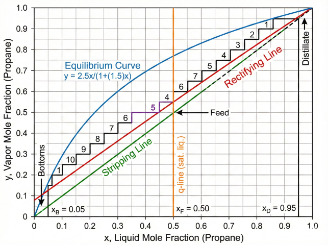
McCabe-Thiele construction for C3/C4 separation: equilibrium curve, operating lines intersecting at q-line, and 11 theoretical stages stepped off from distillate (x_D=0.95) to bottoms (x_B=0.05).
NGL Fractionation
Deethanizer, Depropanizer
Ethane/propane and propane/butane separations in gas plants.
Condensate Stabilization
Light Ends Removal
Remove C1-C2 from condensate to meet RVP specifications.
Debutanizer
LPG Production
C3/C4 overhead (LPG) and C5+ bottoms (natural gasoline).
Preliminary Design
Simulation Input
Quick tray count estimate before rigorous modeling.
Key Definitions
Theoretical stage: Equilibrium stage where vapor and liquid leaving are in thermodynamic equilibrium (Murphree efficiency = 100%)
Equilibrium curve: y vs. x plot from VLE data at column pressure; lies above 45° diagonal for light component enrichment
Operating line: Material balance relating passing vapor (yn+1) and liquid (xn) streams
Reflux ratio (R): L/D where L = reflux returned to column, D = distillate withdrawn
q-line: Feed condition line; intersects 45° line at (zF, zF)
Minimum reflux (Rmin): Reflux ratio where operating line is tangent to equilibrium curve (pinch point)
Fundamental Assumptions
Binary or pseudo-binary: Two components or key component approximation
Constant molal overflow (CMO): L and V constant in each section; valid when latent heats are similar (ΔHvap,A ≈ ΔHvap,B)
Adiabatic operation: No heat loss through column walls
Total condenser: All vapor condensed; xD = y1 (partial condenser requires modification)
Negligible pressure drop: Constant pressure throughout (typically valid for low-pressure columns)
Engineering Value: McCabe-Thiele provides immediate insight into column behavior that simulators cannot—graphical understanding of how R, q, xD, and xB affect stage count. Essential for troubleshooting operating columns, optimizing feed location, and validating simulation results.
2. Equilibrium Curve Construction
The equilibrium curve plots vapor composition (y) versus liquid composition (x) at column pressure—the foundation of McCabe-Thiele design.
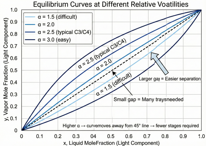
Equilibrium curves at different relative volatilities: higher α moves curve away from 45° diagonal, reducing required stages. α=2.5 typical for C3/C4 separation.
Vapor-Liquid Equilibrium
Relative Volatility Equation:
y = (α × x) / [1 + (α - 1) × x]
Where:
α = K_light / K_heavy = P°_A / P°_B (for ideal systems)
x = liquid mole fraction of light component
y = vapor mole fraction of light component
Physical Interpretation:
α > 1 → Light component enriches in vapor (separation possible)
α = 1 → No separation (equilibrium = 45° line)
α → ∞ → Complete separation in one stage
Temperature/Pressure Effects:
Higher pressure → lower α → harder separation
α varies with composition for non-ideal systems
Typical Relative Volatilities
System
Relative Volatility (α)
Separation Difficulty
Typical Trays
Methane/Ethane (demethanizer)
4.0-6.0
Moderate (cryogenic)
30-50
Ethane/Propane (deethanizer)
3.5-4.5
Moderate
25-40
Propane/Butane (depropanizer)
2.5-3.0
Easy-moderate
15-25
Butane/Pentane (debutanizer)
2.0-2.5
Easy
10-20
Benzene/Toluene
2.3-2.5
Easy
15-25
n-Butane/i-Butane
1.2-1.3
Very difficult
80-120
Ethanol/Water (azeotrope)
1.0 @ 95.6% EtOH
Impossible (azeotrope)
N/A
Generating Equilibrium Data
Method 1: Constant α (most common)
y = (α × x) / [1 + (α - 1) × x]
Use when α varies < ±15% across column.
Method 2: VLE Data Tables
For non-ideal systems, use T-x-y data from:
• Perry's Handbook Chapter 13
• DIPPR database
• Process simulator (Aspen, HYSYS, ProMax)
Method 3: K-Value Charts
y = K_light × x where K = f(T, P)
Use GPSA K-charts or DePriester charts.
Example: Propane/Butane at 200 psia
x (C3)
y (C3)
0.00
0.000
0.20
0.385
0.40
0.625
0.60
0.789
0.80
0.909
1.00
1.000
Based on α = 2.5 (average). Curve lies above 45° line—propane enriches in vapor.
3. Operating Lines & McCabe-Thiele Construction
Operating lines are straight lines representing material balances in the rectifying (above feed) and stripping (below feed) sections. Their slopes depend on internal liquid-to-vapor ratios.
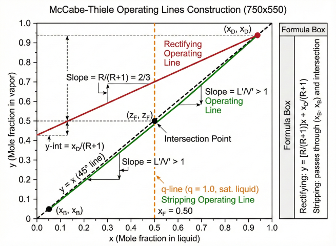
Operating lines construction: rectifying line (slope = R/(R+1)) and stripping line intersect on the q-line at feed composition.
Rectifying Section Operating Line
Rectifying Operating Line:
y = [R/(R+1)] × x + x_D/(R+1)
Where:
R = L/D = Reflux ratio
x_D = Distillate composition (mole fraction light)
Key Points:
• Slope = R/(R+1) — increases with R, approaches 1 as R → ∞
• y-intercept = x_D/(R+1)
• Passes through point (x_D, x_D) on 45° diagonal
• Higher R → steeper line → more stages but better separation
Stripping Section Operating Line
Stripping Operating Line:
Passes through (x_B, x_B) and q-line intersection point.
Slope = L'/V' = (L + qF)/(V - (1-q)F)
Where:
L' = Liquid flow in stripping section
V' = Vapor flow in stripping section
q = Feed liquid fraction
Key Points:
• Slope typically > 1 (steeper than rectifying)
• Always passes through (x_B, x_B) on 45° line
• Intersects rectifying line ON the q-line
Step-by-Step Construction
McCabe-Thiele Step-Off Procedure:
1. Plot equilibrium curve and 45° diagonal
2. Mark x_D, x_F, x_B on x-axis
3. Draw rectifying line from (x_D, x_D) with slope R/(R+1)
4. Draw q-line from (z_F, z_F) with slope q/(q-1)
5. Draw stripping line through (x_B, x_B) and q-line intersection
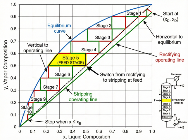
6. Step off stages:
• Start at (x_D, x_D)
• Horizontal to equilibrium curve
• Vertical down to operating line
• Repeat until x ≤ x_B
7. Count steps = N_theoretical (including reboiler as one stage)
Stage step-off procedure: alternate horizontal (to equilibrium) and vertical (to operating line) steps. Feed stage (Stage 5) marks transition from rectifying to stripping section.
Example: C3/C4 Separation
Parameter
Value
Feed (zF)
0.50
Distillate (xD)
0.95
Bottoms (xB)
0.05
α
2.5
q
1.0 (sat. liq.)
R
2.0
Result: 11 theoretical stages, feed at stage 5 from top.
Design Trade-off: Higher R → steeper rectifying line → fewer stages needed BUT higher reboiler/condenser duties. Optimal R typically 1.2–1.5 × Rmin, balancing capital (trays) vs. operating cost (energy).
4. Minimum Reflux Ratio Determination
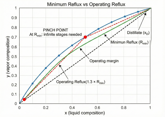
Minimum reflux (Rmin) is the lowest reflux ratio achieving the specified separation—requiring infinite stages. At Rmin, the operating line touches the equilibrium curve at a "pinch point."
Minimum reflux (R_min) creates pinch point requiring infinite stages. Operating at 1.3 × R_min provides margin for finite stage design.
Graphical Method
Finding R_min:
1. Draw q-line from (z_F, z_F)
2. Find q-line / equilibrium curve intersection: (x_p, y_p)
3. Draw line from (x_D, x_D) through (x_p, y_p)
4. Slope = R_min/(R_min+1)
5. Solve: R_min = (x_D - y_p)/(y_p - x_p)
Total Cost Trade-off:
Capital cost ∝ N_trays (column height, diameter)
Operating cost ∝ R (reboiler + condenser duty)
Optimum R = 1.2 to 1.5 × R_min (minimizes total annualized cost)
Rule of thumb: R_opt ≈ 1.3 × R_min for most NGL fractionation
Factors shifting optimum:
- Energy cost (high → favor lower R)
- Equipment cost (high → favor higher R, fewer trays)
- Space constraints (limited height → higher R)
- Existing column (fixed trays → adjust R to meet spec)
Fenske Minimum Stages: At total reflux (R → ∞), minimum stages Nmin = ln[(xD/(1-xD)) × ((1-xB)/xB)] / ln(α). Use Gilliland correlation to relate N and R between these limits.
5. Feed Condition & Actual Trays
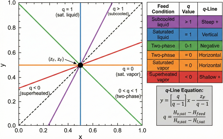
Feed thermal condition (q-value) determines q-line slope and affects stage distribution between rectifying and stripping sections.
q-line orientations depend on feed thermal condition: vertical for saturated liquid (q=1), horizontal for saturated vapor (q=0). Formula: y = [q/(q-1)]x - z_F/(q-1).
Feed Condition Parameter (q)
Definition:
q = (H_sat.vapor - H_feed) / (H_sat.vapor - H_sat.liquid)
q = fraction of feed that is liquid
q-Line Equation:
y = [q/(q-1)] × x - z_F/(q-1)
All q-lines pass through (z_F, z_F) on 45° diagonal.
q-Value Reference
Feed Condition
q
q-Line
Subcooled liquid
> 1
Steep positive
Saturated liquid (bubble pt)
1.0
Vertical
Two-phase
0–1
Negative slope
Saturated vapor (dew pt)
0
Horizontal
Superheated vapor
< 0
Shallow positive
O'Connell Tray Efficiency
Converting Theoretical to Actual Trays:
N_actual = N_theoretical / E_overall
O'Connell Correlation (Perry's 9th Ed.):
E_o = 0.503 × (α × μ_L)^(-0.226)
Where:
μ_L = Liquid viscosity (cP) at column conditions
α = Average relative volatility
Valid range: 0.1 < (α × μ_L) < 10
Typical Efficiencies:
Valve/sieve trays: 60–80%
Low α×μ (< 0.5): E ≈ 75-85%
High α×μ (> 2): E ≈ 50-65%
Design margin: Add 10–20% extra trays for flexibility, fouling, and capacity growth
Feed location: Actual feed nozzle ±1–2 trays from calculated optimal location
Tray spacing: 18–24" typical; 24" for high-pressure or foaming systems
Pressure drop: 0.05–0.15 psi/tray; check reboiler temperature impact
Validate with simulation: Use Aspen HYSYS, ProMax, or Pro/II for final design with actual VLE and tray hydraulics
When to use McCabe-Thiele: Preliminary design, quick estimates, sensitivity analysis, troubleshooting, validating simulator results, and understanding column behavior. For final equipment specifications, always use rigorous simulation.
What is the McCabe-Thiele method for distillation design?+
The McCabe-Thiele method is a graphical technique for determining the number of theoretical stages in a distillation column. It uses the intersection of operating lines and an equilibrium curve to step off stages between the distillate and bottoms compositions.
How is the minimum reflux ratio determined graphically?+
The minimum reflux ratio corresponds to the condition where the operating line pinches against the equilibrium curve, requiring infinite stages. It can be found graphically by drawing the rectifying operating line through the distillate composition tangent to the equilibrium curve, or analytically using the Underwood equation.
What is the feed condition parameter q in McCabe-Thiele?+
The q parameter describes the thermal condition of the feed, ranging from zero for saturated vapor to one for saturated liquid. It determines the slope of the q-line, which locates the intersection of the rectifying and stripping operating lines on the McCabe-Thiele diagram.
How is tray efficiency applied to convert theoretical to actual stages?+
The O'Connell correlation estimates overall tray efficiency based on relative volatility and liquid viscosity. The number of actual trays equals the theoretical stages divided by the tray efficiency, which typically ranges from 50% to 80% for hydrocarbon distillation.