Design and size venturi meters per ISO 5167-4 for applications requiring low permanent pressure loss. Ideal for compressor surge control, high-flow gas measurement, and installations where operating cost matters.
Venturi meters are differential pressure flow measurement devices that offer significantly lower permanent pressure loss than orifice plates. Invented by Giovanni Venturi in 1797 and refined by Clemens Herschel in 1888, they remain the preferred choice for applications where operating cost (compression energy) is critical.
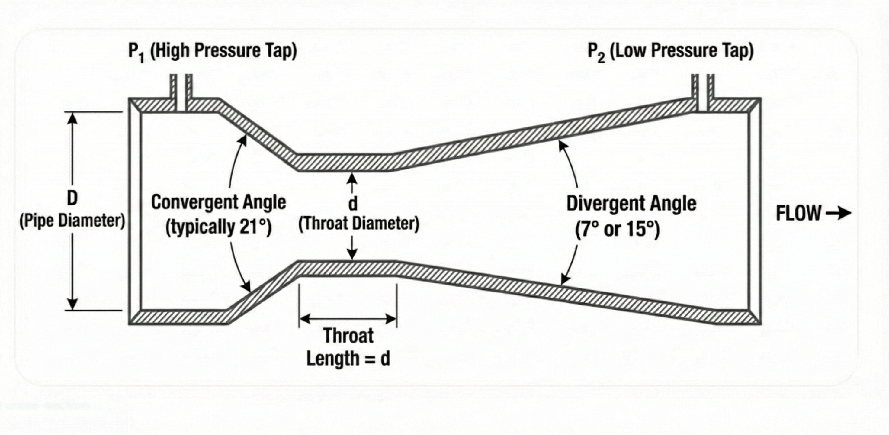
Classical (Herschel) venturi tube: Gradual contraction and expansion minimize turbulence and maximize pressure recovery.
Key advantage
Low permanent loss
10-30% of differential pressure vs 40-90% for orifice. Reduces compression costs.
Discharge coefficient
C = 0.984–0.995
Nearly ideal flow. Much higher than orifice (0.59-0.65).
Disadvantages
Higher cost & length
3-10× orifice cost. Requires more pipe length for installation.
Turndown
3:1 to 5:1
Similar to orifice. Limited by differential pressure transmitter range.
Bernoulli Principle
Like all differential pressure meters, venturis operate on Bernoulli's principle: flow acceleration through the throat creates a pressure drop proportional to velocity squared.
Venturi Flow Equation:
Q = C × ε × (π/4) × d² × √(2 × ΔP / (ρ × (1 - β⁴)))
Where:
Q = Volumetric flow rate (ft³/s or m³/s)
C = Discharge coefficient (0.984-0.995 for classical venturi)
ε = Expansibility factor (gas only)
d = Throat diameter
ΔP = Differential pressure (P₁ - P₂)
ρ = Fluid density at flowing conditions
β = d/D = throat-to-pipe diameter ratio
For incompressible flow (liquids), ε = 1.
For compressible flow (gases), ε accounts for gas expansion.
How a Venturi Works
Convergent section: Flow accelerates gradually (21° cone angle typical) from pipe diameter D to throat diameter d
Throat section: Flow reaches maximum velocity at constant diameter (length = d)
Divergent section: Flow decelerates gradually (7-15° cone angle) back to pipe diameter, recovering most pressure
The gradual transitions minimize flow separation and turbulence, allowing 70-90% of the differential pressure to be recovered—the key advantage over orifice plates.
Standards and Regulations
ISO 5167-4:2003 — Venturi tubes (international standard)
ASME MFC-3M — Measurement of Fluid Flow Using Orifice, Nozzle, and Venturi
API MPMS Ch 14.3 — Natural gas flow measurement (accepts venturi meters)
When to choose venturi over orifice: Select venturi when (1) permanent pressure loss cost over meter lifetime exceeds 3-5× the additional capital cost, (2) application requires very low pressure loss (compressor suction), or (3) installation space allows the longer venturi length.
2. Pressure Recovery Advantage
The venturi's gradual divergent section allows controlled deceleration of flow, converting kinetic energy back to pressure energy. This is the fundamental advantage over orifice plates, where abrupt expansion causes turbulent energy dissipation.
Pressure Recovery vs Orifice
Meter Type
Permanent Loss
Pressure Recovery
Typical Application
Orifice plate
40-90% of ΔP
10-60%
General purpose, custody transfer
Venturi (7° divergent)
10-15% of ΔP
85-90%
Compressor surge control
Venturi (15° divergent)
15-30% of ΔP
70-85%
Space-limited installations
Venturi nozzle (ISA 1932)
30-50% of ΔP
50-70%
High-velocity applications
Flow nozzle
30-80% of ΔP
20-70%
Steam, high temperature
Permanent Pressure Loss Calculation
Permanent Pressure Loss (Classical Venturi):
For 7° divergent angle:
ΔP_perm = ΔP_measured × (0.218 - 0.420β + 0.380β²)
For 15° divergent angle:
ΔP_perm = ΔP_measured × (0.436 - 0.860β + 0.760β²)
Example (β = 0.50, ΔP = 100 in H₂O):
7° divergent:
ΔP_perm = 100 × (0.218 - 0.420×0.5 + 0.380×0.25) = 10.3 in H₂O
Recovery = 89.7%
15° divergent:
ΔP_perm = 100 × (0.436 - 0.860×0.5 + 0.760×0.25) = 19.6 in H₂O
Recovery = 80.4%
Compare to orifice at β = 0.50:
ΔP_perm ≈ 73 in H₂O (73% loss, only 27% recovery)
Operating Cost Impact
For gas compression applications, permanent pressure loss directly increases compression horsepower:
Compression Cost of Permanent Pressure Loss:
Additional HP = (Q × ΔP_perm) / (33,000 × η)
Where:
Q = Flow rate (ACFM)
ΔP_perm = Permanent pressure loss (psi)
η = Compressor efficiency (typically 0.75-0.85)
Example: 50 MMSCFD at 500 psig, 80°F, SG = 0.65
ACFM = 50,000,000 / 1440 × (14.7/514.7) × (540/520) × 0.90 = 927 ACFM
(actual volume = standard × P_std/P × T/T_std × Z)
Orifice (β=0.5): ΔP_meas = 100 in H₂O, ΔP_perm = 100·(1−0.5¹·⁹) = 73 in H₂O = 2.64 psi
Additional HP = (927 × 2.64 × 144) / (33,000 × 0.80) = 13.3 HP
Venturi (β=0.5, 7°): ΔP_meas = 100 in H₂O, ΔP_perm = 10.3 in H₂O = 0.37 psi
Additional HP = (927 × 0.37 × 144) / (33,000 × 0.80) = 1.9 HP
Savings = 11.4 HP continuous
Annual cost savings at $0.10/kWh:
= 11.4 × 0.746 × 8,760 × $0.10 = $7,450/year
Over 20-year meter life: ~$149,000 savings
Divergent Angle Trade-offs
Divergent Angle
Pressure Recovery
Divergent Length
Best Use
5-7°
85-90%
Longest (4-8D)
Maximum recovery, space available
10°
80-85%
Medium (2-4D)
Balanced recovery and length
15°
70-80%
Shortest (1.5-2.5D)
Space-constrained installations
>15°
<70%
Very short
Not recommended (flow separation)
Rule of thumb: If the permanent pressure loss savings over the meter's 20-year life exceed 3-5× the additional capital cost of a venturi vs orifice, choose venturi. For high-pressure gas applications >500 psig, this breakeven point is typically reached at flows >10 MMSCFD.
3. Venturi Geometry & Types
ISO 5167-4 defines two primary venturi types: the Classical (Herschel) Venturi with truncated cone inlet, and the Venturi Nozzle with curved ISA 1932 profile inlet. Each has specific dimensional requirements for calibration validity.
The venturi nozzle combines an ISA 1932 nozzle inlet with a divergent recovery cone. It has a higher pressure loss than the classical venturi but is shorter and has well-characterized performance at high velocities.
Venturi Nozzle Characteristics:
Inlet: Curved ISA 1932 profile (elliptical contraction)
Throat: Cylindrical section, length = 0.3d
Divergent: 7° to 15° cone
Permanent pressure loss: 30-50% (higher than classical)
Discharge coefficient: C = 0.986 to 0.995
Best suited for:
- High-velocity flow (throat velocity >300 ft/s)
- Steam and high-temperature gas
- Shorter installation length required
Discharge Coefficient
The venturi discharge coefficient is much higher and more stable than orifice plates:
Expansibility Factor for Gas Flow (ISO 5167-1, referenced by ISO 5167-4):
Exact isentropic formula (required for venturi tubes):
ε = √{ (κ·τ^(2/κ)/(κ-1)) × ((1-β⁴)/(1-β⁴·τ^(2/κ))) × ((1-τ^((κ-1)/κ))/(1-τ)) }
Where:
τ = p₂/p₁ = (P₁ - ΔP) / P₁ (pressure ratio)
κ = Isentropic exponent (Cp/Cv)
P₁ = Upstream absolute pressure
ΔP = Differential pressure
For natural gas: κ ≈ 1.27-1.31
For air: κ = 1.40
Validity limit: ΔP/P₁ ≤ 0.25
Note: This is NOT the orifice empirical approximation from ISO 5167-2.
The exact formula is required for nozzles (ISO 5167-3) and venturi tubes (ISO 5167-4).
Example: β = 0.50, ΔP = 100 in H₂O = 3.6 psi, P₁ = 500 psia, κ = 1.30
τ = (500 - 3.6)/500 = 0.9928
ε = 0.9956 (from exact formula)
For most gas applications with ΔP/P₁ < 0.05, ε ≈ 0.99-1.00
Pressure Tap Locations
Upstream tap (P₁): Located 0.5D to 1D upstream of convergent entrance
Throat tap (P₂): Located at mid-throat (0.5d from throat entrance)
Tap drilling: 0.25" to 0.50" diameter, perpendicular to wall, flush with inside surface
Multiple taps: 4 taps at 90° intervals, manifolded for averaging (recommended)
Construction quality matters: Machined venturis (C = 0.995) have 40% lower uncertainty than as-cast venturis (C = 0.984). For custody transfer applications, always specify machined or lab-calibrated venturis.
4. Sizing & Calculations
Venturi sizing involves selecting throat diameter to achieve desired differential pressure at design flow while maintaining beta ratio within ISO 5167-4 limits (0.30-0.75).
Sizing Procedure
Venturi Sizing Steps:
Given: Q_design, P, T, gas properties, pipe diameter D
Step 1: Calculate gas density at flowing conditions
ρ = (P × MW) / (Z × R × T)
Step 2: Convert design flow to actual conditions
Q_actual = Q_std × (P_std/P) × (T/T_std) × (Z/Z_std)
Step 3: Select target differential pressure
Typical: 100-200 in H₂O for good accuracy and turndown
Maximum: 400 in H₂O (limited by transmitter range)
Step 4: Assume initial beta (0.50 recommended)
Step 5: Calculate required throat area from flow equation
A = Q / (C × ε × √(2 × ΔP / (ρ × (1 - β⁴))))
Step 6: Calculate throat diameter
d = √(4 × A / π)
Step 7: Calculate actual beta
β = d / D
Step 8: Check 0.30 ≤ β ≤ 0.75; if not, adjust ΔP and repeat
Step 9: Verify Reynolds number
Re_D = 4 × ṁ / (π × D × μ) > 2 × 10⁵
Step 10: Calculate physical dimensions
Example: Size Venturi for Compressor Suction
Given:
Gas flow: 25 MMSCFD natural gas
Suction pressure: 300 psig
Temperature: 80°F
Pipe: 16" Schedule 40 (ID = 15.0")
Gas: SG = 0.65, MW = 18.8, Z = 0.92, κ = 1.28
Target ΔP: 150 in H₂O
Step 1: Gas density
P_abs = 300 + 14.7 = 314.7 psia
T_R = 80 + 460 = 540°R
ρ = (314.7 × 18.8) / (0.92 × 10.73 × 540) = 1.11 lb/ft³
Step 2: Actual flow rate
Q_std = 25,000,000 scfd / 86,400 = 289.4 scfm
Q_actual = 289.4 × (14.73/314.7) × (540/520) × (0.92/1.0)
Q_actual = 289.4 × 0.0468 × 1.038 × 0.92 = 12.93 acfm = 0.216 acfs
Step 3: Assume β = 0.50, C = 0.995, ε = 0.997
ΔP = 150 in H₂O = 5.42 psi = 780 lbf/ft²
Step 4: Required throat area
Velocity factor = √(2 × 780 / (1.11 × (1 - 0.0625))) = √1501 = 38.7 ft/s
A = 0.216 / (0.995 × 0.997 × 38.7) = 0.00563 ft² = 0.810 in²
Step 5: Throat diameter
d = √(4 × 0.810 / π) = 1.015" → Use 1.0" throat? No, too small!
Problem: β = 1.0/15.0 = 0.067 (below minimum 0.30)
Iteration: Reduce ΔP to 50 in H₂O
... (calculations)
Result: d = 7.5", β = 0.50 ✓
Final Design:
Throat diameter: 7.5"
Beta ratio: 0.50
ΔP at design: 50 in H₂O
Permanent loss: 5-7 in H₂O (10-15%)
Divergent angle: 7° (recommended)
Total length: ~5 ft
Beta Ratio Selection Guide
Consideration
Low Beta (0.30-0.45)
Optimal Beta (0.45-0.60)
High Beta (0.60-0.75)
Differential pressure
High ΔP
Moderate ΔP
Low ΔP
Throat velocity
Very high
Moderate
Low
Turndown ratio
4:1 to 5:1
3:1 to 4:1
2:1 to 3:1
Permanent loss
Higher (15-20%)
Low (10-15%)
Lowest (8-12%)
Physical length
Longest
Medium
Shortest
Cost
Highest
Moderate
Lowest
Flow Rate Calculation
Venturi Flow Calculation (from measured ΔP):
Q_MMSCFD = N × C × ε × E_v × d² × √(h_w × P_f / (T_f × SG × Z))
Where:
N = 0.1851 (unit constant for Q in MMSCFD — bundles 2·g_c, R, π/4 and the
14.73 psia / 60°F base; equals 7,713 if Q is in SCFH. This is the
AGA-3 basic-orifice coefficient 338.2 combined with √519.67 from
the temperature/gravity/supercompressibility base factors.)
E_v = 1/√(1 − β⁴) (velocity of approach — REQUIRED, depends on β)
C = Discharge coefficient (≈0.984 classical venturi)
ε = Expansibility factor
d = Throat diameter (inches)
h_w = Differential pressure (inches H₂O)
P_f = Flowing pressure (psia)
T_f = Flowing temperature (°R)
SG = Gas specific gravity
Z = Compressibility factor
Example: D = 12", d = 6" (β = 0.50), h_w = 100 in H₂O, P_f = 514.7 psia,
T_f = 540°R, SG = 0.65, Z = 0.90, C = 0.984, ε = 0.995
E_v = 1/√(1 − 0.50⁴) = 1.033
Q_MMSCFD = 0.1851 × 0.984 × 0.995 × 1.033 × 36 × √(100 × 514.7 / (540 × 0.65 × 0.90))
= 0.1872 × 36 × √(51,470 / 315.9) = 6.74 × 12.77 = 86.0 MMSCFD
Sizing tip: For compressor surge control, size the venturi throat for 110-120% of maximum expected flow at 80% of transmitter range. This provides headroom for flow excursions while maintaining good accuracy in the normal operating range.
5. Applications & Selection
Venturi meters excel in specific applications where their higher capital cost is justified by operating cost savings or technical requirements.
Ideal Applications for Venturi Meters
Compressor suction/surge control: Low pressure loss critical to avoid compressor surge; real-time flow measurement for anti-surge control
High-pressure gas transmission: Permanent loss × pressure × flow = significant compression energy over 20+ year life
Large-diameter pipelines (>24"): Orifice permanent loss becomes prohibitive at high flows
Dirty/erosive fluids: No sharp edges to erode; less sensitive to buildup than orifice
Pulsating flow: More stable than orifice due to higher C and gradual transitions
Wet gas/two-phase: Better handling of liquid droplets due to smooth geometry
Venturi vs Orifice Selection Matrix
Factor
Favor Venturi
Favor Orifice
Permanent pressure loss cost
High (>$50,000/year)
Low (<$10,000/year)
Operating pressure
>500 psig
<200 psig
Flow rate
>20 MMSCFD
<5 MMSCFD
Pipeline diameter
>16"
<8"
Installation space
Available (>10D)
Limited
Fluid cleanliness
Dirty, erosive, wet
Clean, dry
Flow profile
Disturbed, pulsating
Steady, developed
Budget priority
Operating cost
Capital cost
Accuracy requirement
±0.5% (custody)
±1-2% (process)
Installation Requirements
Venturi Installation (ISO 5167-4):
Upstream straight pipe:
- After single 90° elbow: 4D minimum (vs 17D for orifice)
- After two elbows in plane: 7D minimum (vs 34D for orifice)
- After reducer: 4D minimum (vs 22D for orifice)
- After expander: 3D minimum (vs 12D for orifice)
Downstream straight pipe: 4D minimum
Key advantage: Venturi requires only 20-30% of orifice straight pipe length
due to:
- Higher C value less sensitive to velocity profile
- Convergent section acts as flow straightener
Orientation: Horizontal preferred; vertical acceptable with proper draining
Pressure taps: At horizontal plane (±15°) for gas; at bottom for liquid
Cost-Benefit Analysis Template
Venturi vs Orifice Economic Comparison:
Capital Costs:
- Orifice fitting + plate: $5,000 - $15,000 (size dependent)
- Venturi meter: $15,000 - $75,000 (3-5× orifice cost)
- Delta capital: $10,000 - $60,000
Operating Costs (annual compression energy):
- Orifice permanent loss: ΔP_perm × Q × P × 8,760 × electricity_rate / η
- Venturi permanent loss: typically 15-25% of orifice loss
- Annual savings: 75-85% of orifice loss cost
Breakeven calculation:
Years to payback = Delta_capital / Annual_savings
Example: 30 MMSCFD at 800 psig
- Orifice ΔP_perm = 2.5 psi, energy cost = $18,500/year
- Venturi ΔP_perm = 0.4 psi, energy cost = $2,960/year
- Annual savings = $15,540
- Delta capital = $40,000
- Payback = 40,000 / 15,540 = 2.6 years
For 20-year meter life: NPV savings = ~$200,000
Common Venturi Applications by Industry
Natural gas transmission: Main line flow measurement, compressor station metering
Gas processing plants: Inlet separator gas flow, compressor anti-surge control
LNG facilities: Send-out gas measurement, boil-off gas metering
Power generation: Natural gas fuel metering, combustion air measurement
Chemical plants: Process gas flows, reactor feed measurement
Water/wastewater: Large-diameter water mains, pump station monitoring
Bottom line: Choose venturi when permanent pressure loss cost over meter lifetime exceeds 3× the capital cost premium. For high-pressure gas (>500 psig) and large flows (>20 MMSCFD), venturi almost always wins the economic comparison. For low-pressure or small flows, orifice is typically more cost-effective.
What is the pressure recovery advantage of a venturi meter over an orifice plate?+
A venturi meter with a 7° divergent angle recovers 85-90% of the measured differential pressure, resulting in only 10-15% permanent loss. An orifice plate at the same beta ratio loses 40-90% of the differential pressure, making venturis significantly more energy-efficient.
What beta ratio range does ISO 5167-4 specify for venturi meters?+
ISO 5167-4 specifies a beta ratio range of 0.30 to 0.75 for venturi meters. The optimal range is 0.45 to 0.65, which balances measurement accuracy with flow turndown capability.
What is the discharge coefficient of a classical venturi meter?+
The discharge coefficient for a classical (Herschel) venturi ranges from 0.984 to 0.995, which is much higher and more stable than an orifice plate at 0.59-0.65. This near-unity coefficient indicates nearly ideal flow behavior with minimal energy loss.
When should I choose a venturi meter instead of an orifice plate?+
Choose a venturi when permanent pressure loss savings over the meter's 20-year life exceed 3-5× the additional capital cost versus an orifice. Venturis are ideal for compressor surge control, high-flow gas measurement above 10 MMSCFD at pressures over 500 psig, and installations where operating cost matters.
What are the standard divergent cone angles for venturi meters?+
The divergent cone angle is typically 7° for maximum pressure recovery (85-90%) or 15° for shorter installations with moderate recovery (70-80%). Angles above 15° are not recommended because flow separation reduces pressure recovery below 70%.