Measure gas and liquid flow rates using orifice meters with AGA Report 3 and ISO 5167 standards, discharge coefficients, beta ratio optimization, and proper installation practices.
Orifice meters are the most common flow measurement devices in the oil and gas industry. They operate on the Bernoulli principle: a flow restriction creates a pressure drop proportional to the square of the flow rate.
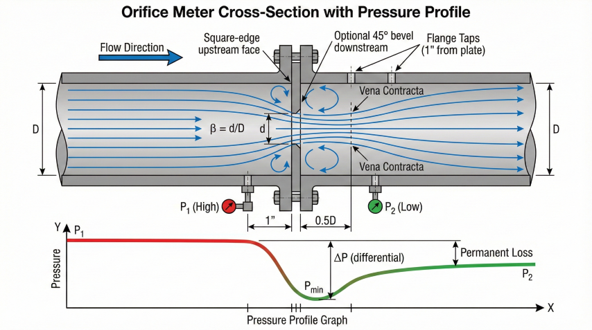
Orifice meter cross-section with pressure profile: Flow accelerates through restriction, creating measurable differential pressure.
Advantages
Simple & proven
No moving parts, low cost, 100+ years of field data, industry standard.
Custody transfer
AGA-3 certified
Accepted for revenue metering when installed per AGA Report 3 or ISO 5167.
Disadvantages
Permanent ΔP loss
50-90% of differential pressure is permanent loss (increases compression cost).
Turndown
3:1 typical
Limited turndown compared to ultrasonic (10:1) or turbine (20:1) meters.
Bernoulli Principle
Bernoulli Equation (Ideal Fluid):
P₁/ρ + v₁²/2 + g×z₁ = P₂/ρ + v₂²/2 + g×z₂
For horizontal flow (z₁ = z₂):
P₁ - P₂ = ρ/2 × (v₂² - v₁²)
Velocity increase at restriction → Pressure decrease
Where:
P = Pressure (psi or Pa)
ρ = Density (lb/ft³ or kg/m³)
v = Velocity (ft/s or m/s)
g = Gravitational acceleration
z = Elevation
Orifice creates velocity increase at vena contracta (minimum flow area).
Orifice Types
Orifice Type
Description
Applications
Concentric square-edge
Sharp 90° upstream edge, centered
Clean gas/liquid, single phase (most common)
Eccentric
Off-center hole (top or bottom)
Two-phase flow, liquids with solids
Segmental
Segment removed from edge
Slurries, high viscosity, solids-laden
Quadrant-edge
Rounded upstream edge (1/4 circle)
Low Reynolds number (Re < 10,000)
Conical entrance
Beveled upstream entry
Low Re, viscous liquids
Tap Configurations
Pressure tap location significantly affects measurement accuracy:
Pressure tap configurations comparison: Flange taps (USA/AGA-3) vs Corner taps (ISO 5167) vs D and D/2 vs Vena Contracta.
Flange taps: 1" upstream, 1" downstream of orifice face (USA standard, AGA-3)
Corner taps: Immediately adjacent to orifice plate faces (European ISO 5167 standard)
D and D/2 taps: 1D upstream, 0.5D downstream (less common)
Vena contracta taps: 1D upstream, 0.3-0.8D downstream at minimum pressure point
Why orifice meters dominate: Despite permanent pressure loss, orifice meters remain the industry standard for custody transfer due to their simplicity, low initial cost, proven accuracy, and widespread acceptance in contracts. Installation costs are typically 1/3 that of ultrasonic meters.
Standards and Regulations
AGA Report 3: Orifice Metering of Natural Gas (USA standard for custody transfer)
ISO 5167: Measurement of fluid flow by means of pressure differential devices (international)
API 14.3 (MPMS Ch 14.3): Orifice Metering of Natural Gas and Other Related Hydrocarbon Fluids
ASME MFC-3M: Measurement of Fluid Flow in Pipes Using Orifice, Nozzle, and Venturi
2. Discharge Coefficient
The discharge coefficient (C or Cd) accounts for real fluid effects: friction, viscosity, flow contraction, and velocity profile. It corrects the theoretical flow equation for actual conditions.
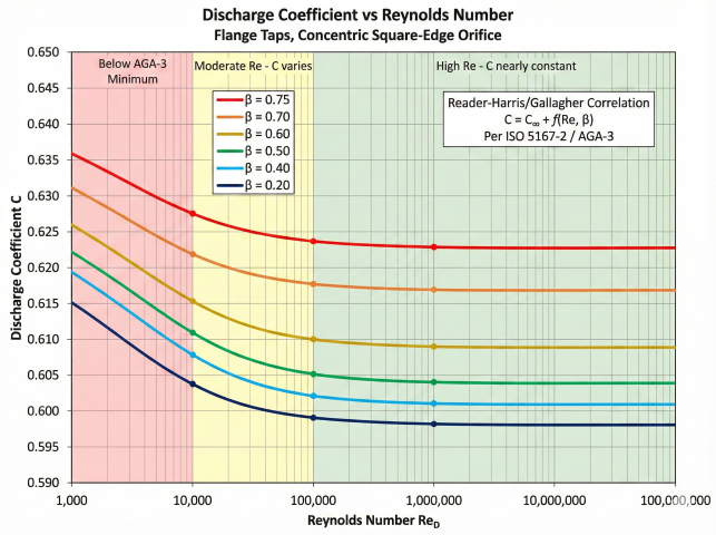
Discharge coefficient vs Reynolds number: C approaches asymptotic value at high Re; higher β gives higher C.
Fundamental Flow Equation
Basic Orifice Equation:
Q = C × E × Y × A × √(2 × g_c × ΔP / ρ)
Where:
Q = Volumetric flow rate (ft³/s or m³/s)
C = Discharge coefficient (dimensionless)
E = Velocity of approach factor = 1/√(1 - β⁴)
Y = Expansion factor (gas only, Y = 1 for liquids)
A = Orifice throat area = π × d² / 4
ΔP = Differential pressure (lbf/ft² = psi×144, or Pa)
ρ = Fluid density at flowing conditions (lbm/ft³ or kg/m³)
g_c = 32.174 lbm·ft/(lbf·s²) in US units; g_c = 1 (omit) in coherent SI
For incompressible flow (liquids), Y = 1.
For compressible flow (gases), Y accounts for gas expansion.
Discharge Coefficient Correlations
C depends on Reynolds number, beta ratio, and tap configuration:
Reader-Harris/Gallagher Equation (1998, ISO 5167):
C = C_∞ + (A₁/Re_D^0.75)
Where:
C_∞ = Asymptotic value at infinite Reynolds number
Re_D = Pipe Reynolds number = ρ × v × D / μ
For flange taps:
C_∞ = 0.5961 + 0.0261β² - 0.216β⁸ + 0.000521(10⁶β/Re_D)^0.7
+ (0.0188 + 0.0063A)β^3.5 × (10⁶/Re_D)^0.3
+ (0.043 + 0.080e^(-10L₁) - 0.123e^(-7L₁))(1 - 0.11A)β⁴/(1 - β⁴)
Where:
A = (19000β/Re_D)^0.8
L₁ = upstream tap distance / D
β = d/D
This is the current AGA-3 (2012) standard correlation.
Accuracy: ±0.5% for 0.10 ≤ β ≤ 0.75, Re_D > 4,000
Typical Discharge Coefficient Values
Beta Ratio
Re_D = 10,000
Re_D = 100,000
Re_D = 1,000,000
β = 0.20
0.5990
0.5980
0.5977
β = 0.40
0.6025
0.6010
0.6005
β = 0.50
0.6070
0.6045
0.6035
β = 0.60
0.6140
0.6100
0.6085
β = 0.70
0.6250
0.6190
0.6165
β = 0.75
0.6340
0.6260
0.6225
Reynolds Number Effects
High Re (> 100,000): C is nearly constant, weak Re dependence, high accuracy
Moderate Re (10,000-100,000): C varies slowly with Re, typical pipeline conditions
Low Re (< 10,000): C decreases rapidly, high uncertainty, not recommended for custody transfer
Velocity of Approach Factor (E):
E = 1 / √(1 - β⁴)
This factor accounts for the upstream velocity before the orifice:
- At β = 0.20: E = 1.0008 (negligible)
- At β = 0.40: E = 1.0131
- At β = 0.50: E = 1.0328
- At β = 0.60: E = 1.0719
- At β = 0.70: E = 1.1471
- At β = 0.75: E = 1.2095
E increases rapidly as β approaches 1.0 (small restriction).
For β < 0.5, E is often omitted as it's close to 1.0.
Expansion Factor for Gas
Expansion Factor (Y) for Compressible Fluids:
Y = 1 - (0.41 + 0.35β⁴) × (ΔP / P₁) / k
Where:
k = Isentropic exponent (Cp/Cv)
P₁ = Upstream absolute pressure
ΔP = Differential pressure (P₁ - P₂)
For natural gas: k ≈ 1.27–1.30
For air: k = 1.40
Limit: ΔP/P₁ < 0.25 for AGA-3 validity
Example:
β = 0.60, ΔP = 100 in H₂O, P₁ = 800 psia, k = 1.27
ΔP/P₁ = (100/27.7)/800 = 0.0045 (well within limit)
Y = 1 - (0.41 + 0.35×0.60⁴) × 0.0045 / 1.27 = 0.9986 ≈ 1.0
For liquid flow: Y = 1.0 (incompressible)
Practical insight: For typical gas pipeline conditions (β = 0.4-0.6, moderate ΔP), the discharge coefficient C dominates uncertainty (±0.5%), while E and Y are close to 1.0 and contribute minimal error. Focus calibration efforts on accurately determining C through Reynolds number calculation.
3. Beta Ratio & Sizing
Beta ratio (β = d/D) is the most important design parameter for orifice meters. It determines differential pressure, accuracy, permanent pressure loss, and turndown capability.
Beta Ratio Trade-offs
Beta Ratio Definition:
β = d / D
Where:
d = Orifice bore diameter (inches or mm)
D = Meter tube inside diameter (inches or mm)
Allowed range per AGA-3: 0.10 ≤ β ≤ 0.75
Recommended range: 0.40 ≤ β ≤ 0.65
Differential Pressure Relationship:
ΔP ∝ 1 / (β⁴ × (1 - β⁴))
For constant flow rate:
- Higher β → Lower ΔP (less sensitive, poor turndown)
- Lower β → Higher ΔP (more sensitive, better turndown)
Beta Ratio Selection Criteria
Consideration
Low Beta (0.20-0.40)
Optimal Beta (0.40-0.65)
High Beta (0.65-0.75)
Differential pressure
Very high ΔP
Moderate ΔP
Low ΔP
Permanent loss
85-90% of ΔP
60-75% of ΔP
50-60% of ΔP
Turndown ratio
5:1 (excellent)
3:1 (good)
2:1 (poor)
Accuracy
±1-2%
±0.5-1%
±1-2%
Re sensitivity
Low
Low
Moderate
Wear/erosion
High (high velocity)
Moderate
Low
Best use
Wide flow range
General purpose
High pressure loss sensitive
Differential Pressure Guidelines
Minimum ΔP: 10 in H₂O (0.036 psi) for reliable transmitter accuracy
Typical ΔP: 50-200 in H₂O (0.18-0.72 psi) for natural gas metering
Maximum ΔP: 500 in H₂O (1.8 psi) or ΔP/P₁ < 0.25, whichever is lower
Optimal ΔP: 100-150 in H₂O provides good accuracy with acceptable permanent loss
Orifice Sizing Procedure
Orifice Bore Diameter Calculation:
Step 1: Determine design flow rate Q_max (maximum expected flow)
Step 2: Select meter tube diameter D (typically same as pipe diameter)
Step 3: Select target differential pressure ΔP_design (e.g., 100 in H₂O)
Step 4: Calculate fluid properties: ρ, μ at flowing P/T
Step 5: Assume initial β (e.g., 0.50)
Step 6: Calculate Re, C, E, Y iteratively
Step 7: Solve for required orifice area:
A = Q / (C × E × Y × √(2 × g_c × ΔP / ρ)) [g_c = 32.174 in US units]
Step 8: Calculate bore diameter:
d = √(4 × A / π)
Step 9: Calculate β = d / D
Step 10: Check 0.40 ≤ β ≤ 0.65; if not, adjust ΔP_design and repeat
Iteration required because C depends on β and Re, which depend on d.
Typically converges in 2-3 iterations.
Permanent Pressure Loss
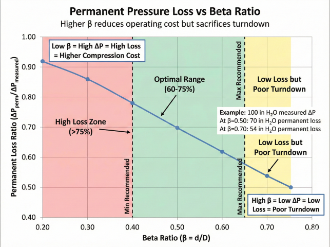
Permanent pressure loss vs beta ratio: Higher β reduces operating cost but sacrifices turndown capability.
Permanent Pressure Loss:
ΔP_permanent = K × ΔP_differential
Where K depends on beta ratio:
- β = 0.20: K = 0.90 (90% permanent loss)
- β = 0.40: K = 0.75
- β = 0.50: K = 0.68
- β = 0.60: K = 0.60
- β = 0.70: K = 0.52
- β = 0.75: K = 0.48
Lower beta → higher permanent loss → higher compression costs
For custody transfer, permanent loss is a significant operating cost over
the meter's 20-30 year lifetime. Consider Venturi or ultrasonic meters
for high-pressure applications where permanent loss cost exceeds equipment cost.
Turndown Ratio
Turndown is the ratio of maximum to minimum measurable flow rate:
Turndown Ratio:
Turndown = Q_max / Q_min
Since ΔP ∝ Q²:
ΔP_max / ΔP_min = (Q_max / Q_min)²
If ΔP_max = 200 in H₂O and ΔP_min = 10 in H₂O (transmitter limit):
ΔP_ratio = 200/10 = 20
Turndown = √20 = 4.47:1
Achieving 5:1 turndown requires:
- Low beta ratio (β < 0.5) for high ΔP at max flow
- Accurate low-range transmitter (±0.1% of reading)
- Maintain Re_D > 4,000 at minimum flow
Optimal beta selection: For most applications, β = 0.50-0.60 provides the best balance: moderate ΔP (100-150 in H₂O), good accuracy (±0.5-1%), acceptable permanent loss (60-70%), and reasonable turndown (3:1). Use β < 0.50 only when wide turndown is required.
Standard Orifice Plate Sizes
Orifice plates are manufactured to standard bore sizes (inches):
Small bores: 0.250, 0.375, 0.500, 0.625, 0.750, 0.875, 1.000
Increments: 1/8" increments from 1" to 2", 1/4" increments from 2" to 4"
Large bores: 1/2" increments above 4"
Custom bores: Available for special applications (add cost, lead time)
Example Sizing Calculation
Size orifice plate for 10 MMscfd natural gas at 800 psia, 80°F in 6" Schedule 40 pipe:
Given:
Q = 10 MMscfd = 6,944 scfm
P₁ = 800 psia, T = 80°F = 540°R
D = 6.065" (6" Sch 40 ID)
Target ΔP = 100 in H₂O = 3.61 psi
SG = 0.65, μ = 0.012 cP, Z = 0.88
Step 1: Convert to actual flow
Q_actual = 6,944 × (14.7/800) × (540/520) × (0.88/1.0) = 116.6 acfm = 1.943 ft³/s
Step 2: Calculate density
ρ = (800 × 0.65 × 28.97) / (0.88 × 10.73 × 540) = 2.95 lb/ft³
Step 3: Assume β = 0.50, calculate C, E, Y
Assume Re ≈ 5×10⁶ (will verify): C ≈ 0.600
E = 1/√(1-0.50⁴) = 1.033
Y = 1 - (0.41 + 0.35×0.50⁴) × (3.61/800) / 1.27 = 0.9985 ≈ 1.0
Step 4: Required orifice area (US units require g_c = 32.174 lbm·ft/lbf·s²)
A = Q / (C × E × Y × √(2 × g_c × ΔP / ρ))
A = 1.943 / (0.600 × 1.033 × 1.0 × √(2 × 32.174 × 3.61 × 144 / 2.95))
A = 1.943 / (0.620 × 106.5) = 0.0294 ft² = 4.24 in²
Step 5: Bore diameter
d = √(4 × 4.24 / π) = 2.32"
Step 6: Actual beta
β = 2.35 / 6.065 = 0.388 (acceptable, but just below the 0.40-0.65 optimal band)
Step 7: To raise β into the optimal range, LOWER the target ΔP to 50 in H₂O, repeat
Results in d = 2.78", β = 0.458 ✓
Select 2.75" bore (nearest standard size)
Final β = 2.75 / 6.065 = 0.453
Final ΔP ≈ 51 in H₂O at design flow
4. Installation Requirements
Proper installation is critical to achieving stated accuracy. AGA Report 3 specifies strict requirements for meter tube straightness, upstream conditioning, and piping configuration to ensure fully developed flow profile.
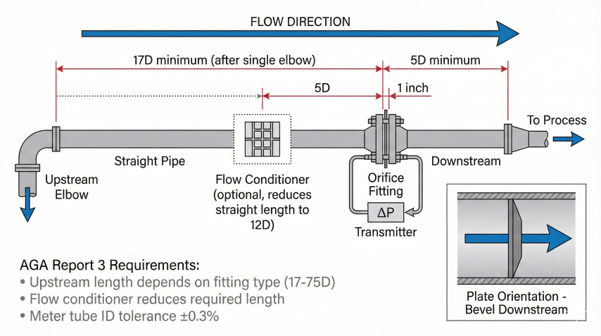
AGA Report 3 installation requirements: Upstream length depends on fitting type (17-75D); flow conditioner reduces required length.
Straight Pipe Requirements
Minimum Straight Pipe Lengths (AGA-3):
Upstream straight pipe: 10D to 75D depending on upstream disturbance
Downstream straight pipe: 5D minimum (not as critical)
Where D = meter tube inside diameter
Specific requirements (most restrictive):
- After single 90° elbow: 17D upstream
- After two 90° elbows in same plane: 34D upstream
- After two 90° elbows in perpendicular planes: 48D upstream
- After reducer (2:1): 22D upstream
- After expander (1:2): 12D upstream
- After control valve: 75D upstream (or use flow conditioner)
Downstream requirement: 5D minimum (up to 8D for high beta)
Straight Length by Beta Ratio
Upstream Fitting
β ≤ 0.50
0.50 < β ≤ 0.60
0.60 < β ≤ 0.75
Straight pipe (ideal)
10D
12D
15D
Single 90° elbow
17D
22D
30D
Two elbows, same plane
34D
40D
50D
Two elbows, perp. planes
48D
55D
65D
Globe valve (fully open)
75D
75D
75D
Flow Conditioners
Flow conditioners reduce required upstream straight length by straightening swirl and normalizing velocity profile:
Tube bundle: 19 or 25 parallel tubes, length = 2D, reduces straight length to 12D after any fitting
Gallagher plate: Perforated plate with specific hole pattern, reduces to 17D minimum
Vane type (Zanker, K-Lab): Helical vanes remove swirl, reduces to 10-12D
Etoile straightener: Star-shaped vanes, good swirl removal, 15D minimum
Installation tip: For retrofit installations where straight pipe is inadequate, a tube bundle flow conditioner installed 5D upstream of the orifice can reduce upstream requirement to 12D total, making many installations feasible. However, add 0.5-1.0 psi pressure drop across conditioner.
Meter Tube Specifications
Meter Tube Requirements (AGA-3):
Diameter tolerance: ±0.3% of nominal diameter
Example: 6" tube (6.065" ID) must be 6.065 ± 0.018"
Roundness: Maximum out-of-round = 0.5% of diameter
Check 4 diameter measurements at 45° intervals
Internal finish: Smooth, no pitting, corrosion, or scale buildup
Surface roughness: Ra < 100 microinches (2.5 microns)
Material: Carbon steel, stainless steel (same as pipeline)
Wall thickness: Schedule 40, 80, or XXH per pressure rating
Avoid: Weld seams, backing rings, internal protrusions within ±5D of orifice
Orifice Plate Inspection
Critical dimensions to verify before installation:
Bore diameter (d): Measure with micrometer at 4 points, ±0.001" tolerance
Edge sharpness: Upstream edge must be square and sharp (no nicks or burrs)
Plate thickness (t): Must satisfy t ≤ 0.05D and t ≤ 2d (thin plate requirement)
Plate flatness: No warping or bending, maximum bow = 0.002" per inch of diameter
Concentricity: Bore centered to within ±0.02" of plate diameter
Upstream face: Smooth, no scratches within 0.1d of bore
Beveled downstream: Optional 45° bevel on downstream side (not upstream)
Orifice Holder Types
Holder Type
Description
Applications
Orifice flange union
Plate held between two flanges
Standard, requires shutdown for plate change
Single chamber fitting
Retractable plate via isolation valve
Allows plate change without shutdown, <16" lines
Dual chamber fitting
Two chambers with switching valves
Hot-swappable plates, no flow interruption
Senior fitting
Slide valve extracts carrier with plate
High-pressure applications, up to 1500 psig
Pressure Tap Installation
Pressure Tap Design (Flange Taps):
Location:
- Upstream tap: 1" upstream of orifice plate face
- Downstream tap: 1" downstream of orifice plate face
Tap hole diameter: 0.25" to 0.50" (6-13 mm)
Tap hole must be perpendicular to pipe wall ±2°
Tap hole must be flush with pipe ID (no burrs or protrusion)
Tap hole must be deburred and smooth
Multiple taps:
- Use 4 taps at 90° intervals, manifolded together (averaging)
- Reduces effect of velocity profile asymmetry
- Required for custody transfer (AGA-3)
Single tap acceptable for non-custody service.
Differential Pressure Transmitter
Range selection: Select transmitter range such that normal ΔP is 50-75% of full scale
Accuracy: ±0.1% of full scale minimum for custody transfer
Impulse lines: Equal length, same elevation, sloped continuously (no pockets)
Condensate legs: For gas service, fill impulse lines with liquid (water or glycol) to prevent gas in lines
Pulsation dampening: Install snubbers or restrict orifices in impulse lines if pressure pulsates >5%
Common Installation Errors
Plate installed backwards: Beveled side must face downstream, not upstream
Insufficient straight pipe: Single biggest source of error; use flow conditioner if needed
Rough internal pipe finish: Scale, rust, weld spatter within meter tube affects velocity profile
Leaking flange gasket: Bypass flow around plate causes under-reading
Damaged orifice edge: Nicks, burrs, or rounded edge from improper handling
Pressure tap blockage: Liquids, solids, or ice in taps causes false ΔP reading
Elevation head not corrected: Condensate leg height difference causes bias in ΔP
5. Flow Calculations & Examples
Complete Flow Calculation Procedure
Step-by-Step Flow Rate Calculation:
Given: ΔP (measured), P₁, T₁, D, d, gas composition or SG
Step 1: Calculate beta ratio
β = d / D
Step 2: Calculate gas density (real gas equation)
ρ = (P × MW) / (Z × R × T)
Step 3: Calculate gas velocity (estimate)
v = Q / (π/4 × D²) [requires iteration]
Step 4: Calculate Reynolds number
Re_D = ρ × v × D / μ
Step 5: Calculate discharge coefficient C
Use Reader-Harris/Gallagher correlation (see Section 2)
Step 6: Calculate velocity of approach factor
E = 1 / √(1 - β⁴)
Step 7: Calculate expansion factor
Y = 1 - (0.41 + 0.35β⁴) × (ΔP/P₁) / k
Step 8: Calculate volumetric flow rate (US units require g_c = 32.174 lbm·ft/lbf·s²)
Q = C × E × Y × (π/4 × d²) × √(2 × g_c × ΔP / ρ)
Step 9: Convert to standard conditions if needed
Q_std = Q_actual × (P₁/P_std) × (T_std/T₁) × (Z₁/Z_std)
Iteration: Steps 3-8 require iteration since v depends on Q, which depends on C,
which depends on Re, which depends on v. Typically converges in 2-3 iterations.
AGA-3 Flow Equation (US Units)
AGA Report 3 Gas Flow Equation:
Q_h = F_b × F_r × Y × F_pb × F_tb × F_tf × F_gr × F_pv × √(h_w × P_f)
F_b = basic orifice factor (contains 338.196·d²·C·E_v at the meter)
F_r = Reynolds-number factor (≈1), Y = expansion factor
F_pb = 14.73/P_b, F_tb = (T_b)/519.67, F_tf = √(519.67/T_f)
F_gr = √(1/G), F_pv = supercompressibility = √(1/Z)
Simplified common form (all base factors bundled into one constant):
Q = 7713 × C × E × Y × d² × √(h_w × P_f / (T_f × G × Z))
Where:
Q = Flow rate (scfh at 14.73 psia, 60°F)
C = Discharge coefficient
E = Velocity of approach factor = 1/√(1 − β⁴)
Y = Expansion factor
d = Orifice diameter (inches)
h_w = Differential pressure (inches of water)
P_f = Flowing pressure (psia)
T_f = Flowing temperature (°R)
G = Gas specific gravity (relative to air)
Z = Compressibility factor
7713 = full SCFH constant (incorporates 2·g_c, R, π/4 and the 14.73 psia/60°F base).
It equals the AGA-3 basic-orifice coefficient 338.2 combined with the √519.67 that
the F_tf/F_gr/F_pv base factors contribute — using 338.2 directly in this grouped
form under-predicts by √519.67 ≈ 22.8×. (For MMSCFD, divide by 1×10⁶/24: N = 0.1851.)
Liquid Flow Equation (Incompressible)
Liquid Orifice Flow Equation:
Q = C × E × (π/4 × d²) × √(2 × g_c × ΔP / ρ) [g_c = 32.174 in US units]
Where Y = 1 (incompressible)
In US oilfield units:
Q_bpd = 6,760 × C × E × d² × √(ΔP / (SG × G_L))
Where:
Q_bpd = Liquid flow rate (barrels per day)
d = Orifice diameter (inches)
ΔP = Differential pressure (psi)
SG = Liquid specific gravity (water = 1.0)
G_L = Liquid gravity correction factor ≈ 1.0
For water (SG = 1.0) at 60°F:
Q_gpm = 5.667 × C × E × d² × √ΔP_psi
Uncertainty Analysis
Total measurement uncertainty combines individual parameter uncertainties:
Parameter
Typical Uncertainty
Effect on Flow Rate
Discharge coefficient C
±0.5%
±0.5%
Orifice diameter d
±0.02%
±0.04% (×2)
Meter tube diameter D
±0.3%
±0.1% (via β)
Differential pressure ΔP
±0.1% of span
±0.05% (×0.5)
Flowing pressure P
±0.05% of reading
±0.025% (×0.5)
Flowing temperature T
±1°F
±0.2%
Gas composition (SG)
±0.5%
±0.25% (×0.5)
Compressibility Z
±0.1%
±0.05% (×0.5)
Total Uncertainty (RSS Method):
σ_total = √(σ₁² + σ₂² + ... + σₙ²)
For well-installed meter with calibrated instruments:
σ_total ≈ √(0.5² + 0.04² + 0.1² + 0.05² + 0.025² + 0.2² + 0.25² + 0.05²)
σ_total ≈ ±0.61%
Practical range: ±0.5% to ±2.0% depending on installation quality
Example 1: Natural Gas Flow Calculation
Given:
Meter tube: 8" Schedule 40 (D = 7.981")
Orifice plate: d = 4.500"
Measured ΔP = 125 in H₂O
Flowing pressure P₁ = 850 psia
Flowing temperature T₁ = 75°F = 535°R
Gas SG = 0.60, Z = 0.90, μ = 0.0115 cP, k = 1.28
Step 1: Beta ratio
β = 4.500 / 7.981 = 0.564
Step 2: Gas density
ρ = (850 × 0.60 × 28.97) / (0.90 × 10.73 × 535) = 2.86 lb/ft³
Step 3: Initial C estimate (assume Re = 1×10⁷)
C ≈ 0.605 (from Reader-Harris/Gallagher)
Step 4: E and Y factors
E = 1/√(1 - 0.564⁴) = 1.054
ΔP_psi = 125/27.7 = 4.51 psi
Y = 1 - (0.41 + 0.35×0.564⁴) × (4.51/850) / 1.28 = 0.9981
Step 5: Calculate flow rate (US units require g_c = 32.174 lbm·ft/lbf·s²)
Q = 0.605 × 1.054 × 0.9981 × (π/4 × (4.5/12)²) × √(2 × 32.174 × 4.51 × 144 / 2.86)
Q = 0.637 × 0.1105 × 120.9 = 8.51 ft³/s = 510.6 cfm actual
Step 6: Convert to standard conditions
Q_std = 510.6 × (850/14.73) × (520/535) × (0.90/1.0)
Q_std = 510.6 × 57.7 × 0.972 × 0.90 = 25,770 scfm = 37.1 MMscfd
Step 7: Verify Reynolds number
v = Q / (π/4 × D²) = 8.51 / (π/4 × (7.981/12)²) = 24.5 ft/s
Re = ρ × v × D / μ = 2.86 × 24.5 × (7.981/12) / (0.0115 × 6.72×10⁻⁴) = 6.0×10⁶ ✓
Final answer: Q = 37.1 MMscfd (37 MMscfd rounded)
Example 2: Liquid Flow Calculation
Given:
Meter tube: 6" Schedule 40 (D = 6.065")
Orifice plate: d = 3.000"
Measured ΔP = 45 psi
Liquid: Crude oil, SG = 0.88, μ = 15 cP
Step 1: Beta ratio
β = 3.000 / 6.065 = 0.495
Step 2: Liquid density
ρ = 0.88 × 62.4 = 54.9 lb/ft³
Step 3: E factor (Y = 1 for liquids)
E = 1/√(1 - 0.495⁴) = 1.031
Step 4: Estimate velocity and Re
Assume v ≈ 13 ft/s: Re = ρ × v × D / μ
Re = 54.9 × 13 × 6.065 / (15 × 6.72×10⁻⁴ × 12) = 3.6×10⁴
Step 5: Calculate C (using Reader-Harris for Re = 3.6×10⁴)
C ≈ 0.604
Step 6: Calculate flow rate (US units require g_c = 32.174 lbm·ft/lbf·s²)
Q = 0.604 × 1.031 × (π/4 × (3/12)²) × √(2 × 32.174 × 45 × 144 / 54.9)
Q = 0.623 × 0.0491 × 87.16 = 2.666 ft³/s
Convert to bbl/day:
Q = 2.666 ft³/s × 86,400 s/day / 5.615 ft³/bbl = 41,030 bbl/day
Final answer: Q = 41,000 bbl/day
Troubleshooting Common Issues
Flow rate too high (under-measuring ΔP): Check for tap blockage, condensate leg imbalance, transmitter zero error
Flow rate too low (over-measuring ΔP): Check for bypass leak around plate, damaged orifice edge, wrong plate installed
Erratic readings: Flow pulsation, upstream disturbance, liquid slugs in gas line, gas bubbles in liquid line
Accuracy degradation over time: Orifice erosion (high velocity), buildup on plate (dirty fluids), pipe roughness increase
Low Reynolds number: Increase ΔP by using smaller orifice, heat fluid to reduce viscosity, accept lower accuracy
Calibration and verification: For custody transfer, orifice meters should be verified annually by inspecting the plate for wear/damage and confirming bore diameter. Replace plate if diameter has changed by more than 0.1% or edge is damaged. Recertify differential pressure transmitter every 6-12 months.