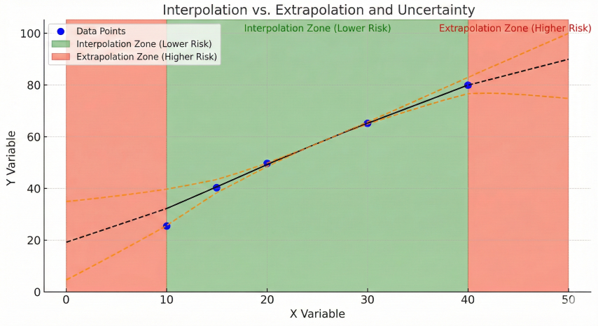
Extrapolation is the process of estimating values beyond the range of known data points. Unlike interpolation (estimating within the data range), extrapolation inherently carries higher uncertainty because it assumes the mathematical relationship continues beyond the observed region.
Property estimation
Physical properties
Viscosity, density, vapor pressure at temperatures outside measured range.
Trend forecasting
Time series data
Production decline curves, corrosion rate projections, demand forecasts.
Calibration curves
Instrument extension
Extending calibration beyond measured points with caution.
Economic analysis
Cost projections
Scaling costs to larger/smaller sizes based on historical data.
Interpolation vs. Extrapolation
Aspect
Interpolation
Extrapolation
Definition
Estimate values within data range
Estimate values outside data range
Accuracy
High (typically ±1-5%)
Lower (±10-50% or worse)
Reliability
Bounded by known data
Assumes trend continues
Risk
Low—values constrained
High—unbounded uncertainty
Engineering use
Standard practice
Use with caution, validate if possible
Interpolation vs extrapolation comparison showing how uncertainty increases rapidly when estimating values beyond the known data range
When Extrapolation is Necessary
Limited experimental data: Property measurements expensive or impractical for full operating range
Emergency scenarios: Need to estimate system behavior at conditions not normally encountered
Design for future expansion: Sizing equipment for throughput beyond current capability
Historical trend analysis: Forecasting production, decline curves, or degradation rates
Proprietary data gaps: Vendor data available only for standard conditions, not extreme cases
Fundamental limitation: Extrapolation assumes the underlying mathematical relationship (linear, polynomial, exponential, etc.) continues beyond the known data. In reality, physical systems often change behavior at boundaries—phase changes, chemical reactions, mechanical limits. Always validate extrapolated results with theoretical limits and subject matter expertise.
Best Practices for Extrapolation
Minimize extrapolation distance: Stay as close to known data as possible
Understand the physics: Use theory to guide method selection (linear, exponential, power law)
Validate with multiple methods: Compare linear, polynomial, exponential—agreement increases confidence
Check physical limits: Ensure extrapolated values don't violate conservation laws or material limits
Quantify uncertainty: Report confidence intervals or error estimates
Test experimentally if critical: For high-stakes applications, measure data points in extrapolated region
Apply safety margins: Design with conservatism to account for extrapolation uncertainty
2. Extrapolation Methods
Selection of extrapolation method depends on data behavior, physical principles, and required accuracy. Common approaches range from simple linear to complex nonlinear models.
Linear Extrapolation
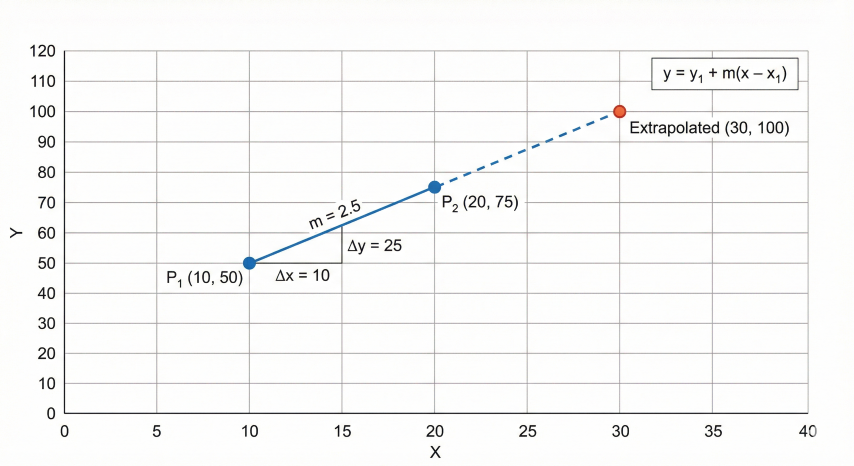
Linear Extrapolation (Two-Point Method):
Simplest method: fit straight line through last two data points.
y = y₁ + [(y₂ - y₁)/(x₂ - x₁)] × (x - x₁)
Where:
(x₁, y₁) = Second-to-last data point
(x₂, y₂) = Last data point
x = Point to extrapolate to
y = Extrapolated value
Slope (m):
m = (y₂ - y₁) / (x₂ - x₁)
Extrapolated value:
y = y₂ + m × (x - x₂)
Example:
Given points: (10, 50) and (20, 75)
Extrapolate to x = 30
m = (75 - 50) / (20 - 10) = 2.5
y = 75 + 2.5 × (30 - 20) = 75 + 25 = 100
Advantages: Simple, conservative for short distances
Disadvantages: Ignores curvature, poor for nonlinear data
Two-point linear extrapolation demonstrating the simplest method for estimating values beyond known data using constant slope
Linear Regression (Least Squares)
Linear Least Squares Fit (Multiple Points):
Fit straight line to all available data using least squares method:
y = a + b × x
Coefficients calculated from n data points (x_i, y_i):
b = [n × Σ(x_i × y_i) - Σx_i × Σy_i] / [n × Σx_i² - (Σx_i)²]
a = [Σy_i - b × Σx_i] / n
Or equivalently:
b = Cov(x,y) / Var(x)
a = ȳ - b × x̄
Where:
ȳ = mean of y values
x̄ = mean of x values
Correlation coefficient (R²):
R² = [Σ(ŷ_i - ȳ)²] / [Σ(y_i - ȳ)²]
R² = 1.0: Perfect linear fit
R² > 0.95: Good linear relationship (reliable for short extrapolation)
R² < 0.80: Poor linear fit (consider nonlinear method)
Example calculation:
Data: (1,2), (2,5), (3,7), (4,10), (5,12)
n = 5
Σx_i = 15, Σy_i = 36, Σ(x_i × y_i) = 133, Σx_i² = 55
(Σx·y = 1·2 + 2·5 + 3·7 + 4·10 + 5·12 = 2 + 10 + 21 + 40 + 60 = 133)
b = [5×133 - 15×36] / [5×55 - 15²] = [665 - 540] / [275 - 225] = 125/50 = 2.5
a = [36 - 2.5×15] / 5 = [36 - 37.5] / 5 = -0.3
Fitted equation: y = -0.3 + 2.5x
Extrapolate to x = 7:
y = -0.3 + 2.5 × 7 = 17.2
Polynomial Extrapolation
Polynomial Fit (2nd or 3rd Order):
For data with curvature, fit polynomial:
2nd order (quadratic):
y = a + b×x + c×x²
3rd order (cubic):
y = a + b×x + c×x² + d×x³
Coefficients determined by least squares minimizing:
S = Σ[y_i - (a + b×x_i + c×x_i² + ...)]²
Solution requires matrix algebra (normal equations):
[A]ᵀ[A]{β} = [A]ᵀ{y}
Where [A] is design matrix:
[A] = [1 x₁ x₁² ...]
[1 x₂ x₂² ...]
[... ... ... ...]
Solving gives coefficients {β} = {a, b, c, ...}
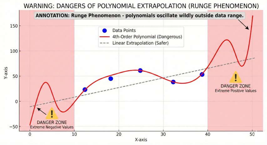
Higher order polynomials (4th, 5th) can fit data more closely but:
- Risk overfitting (fitting noise rather than trend)
- Oscillate wildly outside data range (Runge phenomenon)
- Physically unrealistic behavior
General rule: Use lowest order polynomial that adequately fits data
- Linear: R² > 0.95
- Quadratic: If residuals show systematic curvature
- Cubic: Rarely needed; may indicate need for different model form
Example: Viscosity vs temperature
Data shows exponential decay—polynomial will fail at extrapolation.
Better to use exponential or Arrhenius form.
Polynomial extrapolation pitfall (Runge phenomenon) showing how high-order polynomials oscillate wildly outside the data range while linear extrapolation remains stable
Exponential Extrapolation
Exponential Growth/Decay:
Many physical phenomena follow exponential relationships:
y = a × exp(b × x)
Taking natural logarithm:
ln(y) = ln(a) + b × x
This is linear in ln(y) vs x. Perform linear regression on transformed data:
ln(y) = A + B × x
Where:
A = ln(a) → a = exp(A)
B = b
Then extrapolate using:
y_extrap = a × exp(b × x_extrap)
Common applications:
- Vapor pressure (Antoine equation): log(P) = A - B/(T+C)
- Radioactive decay: N(t) = N₀ × exp(-λt)
- Production decline: q(t) = q_i × exp(-D×t)
- Corrosion penetration: d(t) = d₀ × exp(k×t)
Example: Production decline curve
Data: (0 yr, 1000 bbl/d), (1 yr, 850 bbl/d), (2 yr, 720 bbl/d)
Transform to ln(q) vs t:
(0, 6.908), (1, 6.745), (2, 6.579)
Linear fit: ln(q) = 6.908 - 0.164×t
Therefore: q = 1000 × exp(-0.164×t)
Extrapolate to t = 5 years:
q(5) = 1000 × exp(-0.164×5) = 1000 × exp(-0.82) = 440 bbl/d
Decline rate: D = 0.164 per year = 16.4% annual decline
Power Law Extrapolation
Power Law Relationship:
Form: y = a × x^b
Taking logarithm:
log(y) = log(a) + b × log(x)
Linear in log-log space. Perform regression on log(y) vs log(x):
log(y) = A + B × log(x)
Where:
A = log(a) → a = 10^A
B = b (exponent)
Applications:
- Equipment cost scaling: Cost₂ = Cost₁ × (Size₂/Size₁)^n (n ≈ 0.6-0.8)
- Pipe friction (turbulent): ΔP ∝ Q^1.8
- Heat transfer: Nu ∝ Re^n (n = 0.8 typical)
- Pump power: HP ∝ Q × H (flow × head)
Example: Compressor cost scaling
20,000 HP compressor costs $10 million
Estimate cost of 35,000 HP unit
Assume power law with exponent n = 0.7 (typical for rotating equipment):
Cost₂ = Cost₁ × (HP₂/HP₁)^0.7
Cost₂ = $10M × (35,000/20,000)^0.7
Cost₂ = $10M × (1.75)^0.7 = $10M × 1.47 = $14.7M
Note: Extrapolation to 2× size may not be valid—verify with vendors.
Method Selection Guidelines
Data Behavior
Recommended Method
Example Applications
Constant rate of change
Linear extrapolation
Temperature vs altitude, calibration curves
Slight curvature
Quadratic polynomial
Pressure drop vs flow (moderate range)
Exponential growth/decay
Exponential fit
Decline curves, vapor pressure, reaction kinetics
Power law scaling
Log-log regression
Equipment costs, friction factors, heat transfer
Asymptotic behavior
Logarithmic or hyperbolic
Adsorption isotherms, learning curves
Complex curvature
Spline or physics-based model
Thermodynamic properties (use EOS, not polynomial)
Physics-based models preferred: When available, use theoretical models (equations of state, Antoine equation, Arrhenius law) rather than empirical polynomial fits. Physics-based models extrapolate more reliably because they capture underlying mechanisms. Empirical fits are data interpolators that fail outside calibration range.
3. Statistical Validation
Statistical measures quantify goodness-of-fit and provide confidence intervals for extrapolated predictions. Understanding uncertainty is critical for engineering decisions based on extrapolated data.
Coefficient of Determination (R²)
R² (R-Squared) Value:
Measures proportion of variance in y explained by regression model:
R² = 1 - (SS_res / SS_tot)
Where:
SS_res = Σ(y_i - ŷ_i)² = Sum of squared residuals (unexplained variance)
SS_tot = Σ(y_i - ȳ)² = Total sum of squares (total variance)
ŷ_i = Predicted value from model
ȳ = Mean of observed y values
Interpretation:
R² = 1.0 (100%): Perfect fit, all variance explained
R² = 0.95: 95% of variance explained, 5% unexplained (good fit)
R² = 0.80: 80% explained (fair fit, extrapolation risky)
R² < 0.50: Poor fit, model does not capture relationship
Note: R² always increases with additional polynomial terms, even if overfitting.
Use adjusted R² to penalize excessive parameters:
R²_adj = 1 - [(1 - R²) × (n - 1) / (n - p - 1)]
Where:
n = Number of data points
p = Number of parameters (excluding intercept)
Prefer model with highest R²_adj, not highest R².
Standard Error of Estimate
Standard Error (S_e):
Measures typical deviation of data points from fitted curve:
S_e = √[Σ(y_i - ŷ_i)² / (n - p)]
Where:
n = Number of data points
p = Number of parameters in model (2 for linear: slope + intercept)
Units of S_e are same as y (the dependent variable).
Interpretation:
- Approximately 68% of data points fall within ±S_e of fitted curve
- Approximately 95% fall within ±2×S_e
For extrapolation, standard error increases with distance from data:
S_extrap = S_e × √[1 + 1/n + (x_extrap - x̄)² / Σ(x_i - x̄)²]
Uncertainty grows rapidly as x_extrap moves away from mean x̄.
Example:
Linear fit to 10 data points, S_e = 2.5 units
x̄ = 50, Σ(x_i - x̄)² = 1000
At x_extrap = 60:
S_extrap = 2.5 × √[1 + 0.1 + (60-50)²/1000]
S_extrap = 2.5 × √[1 + 0.1 + 0.1] = 2.5 × 1.095 = 2.74 units
At x_extrap = 100 (far from data):
S_extrap = 2.5 × √[1 + 0.1 + (100-50)²/1000]
S_extrap = 2.5 × √[1 + 0.1 + 2.5] = 2.5 × 1.90 = 4.75 units
Uncertainty nearly doubles when extrapolating twice as far from mean.
Confidence Intervals
Confidence Interval for Extrapolated Value:
95% confidence interval:
y_extrap ± t_α/2 × S_extrap
Where:
t_α/2 = Student's t-value for desired confidence level and (n-p) degrees of freedom
α = 0.05 for 95% confidence (two-tailed)
For large sample (n > 30): t_0.025 ≈ 1.96 ≈ 2.0
For small sample (n = 10): t_0.025 ≈ 2.26
For very small (n = 5): t_0.025 ≈ 2.78
Example (continuing previous):
n = 10, so df = n - p = 10 - 2 = 8
t_0.025,8 = 2.31 (from t-table)
At x = 60:
y_extrap = 125 (from model)
95% CI = 125 ± 2.31 × 2.74 = 125 ± 6.3
Range: 118.7 to 131.3
At x = 100:
y_extrap = 220
95% CI = 220 ± 2.31 × 4.75 = 220 ± 11.0
Range: 209 to 231
Relative uncertainty:
At x=60: ±5% relative error
At x=100: ±5% relative error (same in this case, but absolute error doubled)
For engineering design: Use upper/lower confidence limit as conservative value.
Residual Analysis
Plotting residuals (y_i - ŷ_i) reveals model inadequacies:
Residual Pattern
Interpretation
Corrective Action
Random scatter around zero
Good fit, model captures relationship
Model is appropriate
Systematic curvature (U-shape)
Model is too simple, missing nonlinearity
Add quadratic term or try exponential
Funnel shape (increasing spread)
Heteroscedasticity (non-constant variance)
Use weighted regression or log transform
Outliers (few points far from zero)
Measurement errors or unusual conditions
Investigate and possibly exclude outliers
Trends with x or ŷ
Model bias, systematic error
Try different functional form
Cross-validation technique: For critical extrapolations, withhold last data point(s) from regression, fit model to remaining data, then compare prediction to withheld point. If error is acceptable, model is validated for short extrapolation. If large error, model is unreliable outside data range. Repeat with multiple withheld points (k-fold cross-validation) for robust assessment.
4. Accuracy Assessment
Quantifying extrapolation error is essential for risk management. Accuracy degrades with extrapolation distance and depends on data quality, model appropriateness, and physical behavior.
Factors Affecting Extrapolation Accuracy
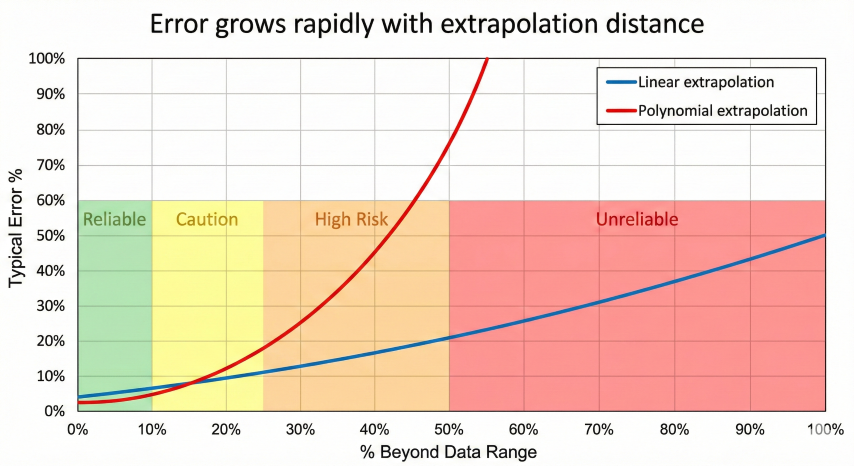
Distance beyond data range: Error grows exponentially with extrapolation distance
Data quality: Measurement errors, outliers, and noise propagate into extrapolated values
Number of data points: More data (n > 10) provides better statistical confidence
Data spacing: Uniform spacing preferred; gaps near extrapolation region increase uncertainty
Model appropriateness: Wrong functional form (linear vs exponential) causes large errors
Error growth versus extrapolation distance showing how polynomial extrapolation error increases much faster than linear, with risk zones from reliable to unreliable
Engineering Safety Margins
Applying Safety Factors to Extrapolated Values:
For design based on extrapolated data, apply safety margin:
Conservative estimate (upper bound):
y_design = y_extrap × (1 + SF)
Or:
y_design = y_extrap + k × S_extrap
Where:
SF = Safety factor (0.10 to 0.50 typical)
k = Number of standard deviations (1.96 for 95% confidence, 2.58 for 99%)
Safety factor selection:
- Low consequence, short extrapolation (10%): SF = 0.10-0.15
- Moderate consequence, moderate extrapolation (25%): SF = 0.20-0.30
- High consequence, long extrapolation (50%): SF = 0.40-0.50
- Critical application (pressure vessel burst): Obtain actual data, avoid extrapolation
Example:
Extrapolated vapor pressure: P_extrap = 250 psia at T = 400°F
Standard error: S_extrap = 20 psia
Design for relief valve set pressure (safety-critical):
Conservative design pressure:
P_design = 250 + 2.58 × 20 = 250 + 52 = 302 psia
Select PSV set pressure: 300 psig (closest standard)
This accounts for extrapolation uncertainty with 99% confidence.
Common Extrapolation Pitfalls
Polynomial oscillation: High-order polynomials oscillate wildly outside data range (Runge phenomenon)
Ignoring physical limits: Extrapolation predicts negative density or temperatures below absolute zero
Assuming linearity: Most physical properties are nonlinear; linear extrapolation oversimplifies
Sparse data: Extrapolating from 2-3 points has very low confidence
When extrapolation fails catastrophically: The 1986 Challenger disaster is a tragic example of extrapolation failure. Engineers extrapolated O-ring performance to 28°F launch temperature based on data at 53°F+. The O-rings behaved completely differently (brittle failure) at the extrapolated temperature, causing loss of crew. Lesson: Never extrapolate safety-critical systems without understanding physical mechanisms.
5. Engineering Applications
Property Estimation Beyond Measured Range
Common scenario: Viscosity measured at 100-200°F, need value at 250°F for pump sizing.
Example: Crude Oil Viscosity Extrapolation
Measured data (kinematic viscosity):
T = 100°F: ν = 45 cSt
T = 150°F: ν = 18 cSt
T = 200°F: ν = 9 cSt
Extrapolate to T = 250°F
Method 1: Linear on ln(ν) vs 1/T (Arrhenius-like):
Transform data:
(1/560°R, ln(45)) = (0.001786, 3.807)
(1/610°R, ln(18)) = (0.001639, 2.890)
(1/660°R, ln(9)) = (0.001515, 2.197)
Linear fit: ln(ν) = A + B × (1/T)
Using regression: B = 5963, A = -6.858
At T = 250°F = 710°R:
ln(ν) = -6.858 + 5963 × (1/710) = -6.858 + 8.398 = 1.540
ν = exp(1.540) = 4.66 cSt
Result appears reasonable, but simple Arrhenius fit is unreliable
for crude oil viscosity extrapolation.
Method 2: Power law ν ∝ T^n
log(ν) vs log(T) regression gives similar estimate (~5 cSt).
For crude oil, always use industry correlations (ASTM D341) rather
than simple extrapolation. Viscosity is highly nonlinear and
varies greatly with crude composition.
Result: At 250°F, estimated ν ≈ 5-6 cSt (using ASTM D341).
Lesson: For thermophysical properties, use established correlations
(Antoine, Wagner, DIPPR) rather than empirical polynomial fits.
Production Decline Curve Forecasting
Example: Oil Well Production Forecast
Historical production:
Year 0: 800 bbl/d
Year 1: 680 bbl/d
Year 2: 580 bbl/d
Year 3: 495 bbl/d
Fit exponential decline: q(t) = q_i × exp(-D×t)
Transform: ln(q) = ln(q_i) - D×t
Regression on ln(q) vs t:
Points: (0, 6.685), (1, 6.522), (2, 6.363), (3, 6.205)
Slope: D = (6.205 - 6.685) / 3 = -0.160 per year
Intercept: ln(q_i) = 6.685 → q_i = 798 bbl/d ✓
Decline equation: q(t) = 798 × exp(-0.160×t)
Extrapolate to Year 5:
q(5) = 798 × exp(-0.160×5) = 798 × 0.449 = 358 bbl/d
Cumulative production to Year 5:
Q_cum = ∫q(t)dt = (q_i / D) × [1 - exp(-D×t)]
Q_cum = (798 / 0.160) × [1 - exp(-0.8)]
Q_cum = 4988 × 0.551 = 2748 bbl/d·yr
Converting to cumulative barrels:
2748 × 365 = 1,003,020 bbl ≈ 1.0 MMbbl cumulative over 5 years
Uncertainty: Production decline can deviate from exponential due to
well interventions, reservoir heterogeneity, water breakthrough.
Apply ±20-30% uncertainty to long-term forecasts.
Equipment Cost Scaling
Example: Compressor Package Cost Estimation
Known costs:
10,000 HP compressor: $6.5 million
25,000 HP compressor: $12.0 million
Estimate cost of 40,000 HP unit (extrapolation beyond data)
Power law fit: Cost = a × HP^b
Taking logs: log(Cost) = log(a) + b × log(HP)
Two-point fit:
log(12.0) - log(6.5) = b × [log(25000) - log(10000)]
1.079 - 0.813 = b × [4.398 - 4.000]
0.266 = b × 0.398
b = 0.668 (exponent, typical for rotating equipment 0.6-0.8)
log(a) = 0.813 - 0.668 × 4.000 = 0.813 - 2.672 = -1.859
a = 10^(-1.859) = 0.0138
Cost equation: Cost = 0.0138 × HP^0.668
For 40,000 HP:
Cost = 0.0138 × (40,000)^0.668
Cost = 0.0138 × 1,187 = $16.4 million
Note: This is 60% beyond data range (25,000 to 40,000 HP).
Apply ±30% uncertainty: $16.4M ± $5M = $11-21M range
For detailed project budgeting, obtain vendor quotes rather than
relying on extrapolation. Use extrapolation for preliminary screening only.
Calibration Curve Extension
Flow meter calibration performed at 50, 100, 150 gpm. Need to operate at 200 gpm.
Calibration data (differential pressure vs flow):
Q = 50 gpm → ΔP = 12 in H₂O
Q = 100 gpm → ΔP = 45 in H₂O
Q = 150 gpm → ΔP = 98 in H₂O
Orifice relationship: Q = C × √(ΔP)
Or: ΔP = K × Q²
Fit ΔP = K × Q²:
K = ΔP / Q²
K₁ = 12 / 50² = 0.00480
K₂ = 45 / 100² = 0.00450
K₃ = 98 / 150² = 0.00436
K decreases slightly with flow rate (discharge coefficient effects).
Average: K_avg = 0.00455
Extrapolate to Q = 200 gpm:
ΔP = 0.00455 × 200² = 0.00455 × 40,000 = 182 in H₂O
However, extrapolation is 33% beyond data. Discharge coefficient
may continue to change. Uncertainty: ±10-15%
Conservative approach:
Use highest K from data: K = 0.00480
ΔP_max = 0.00480 × 40,000 = 192 in H₂O
Size transmitter for 200 in H₂O range with 10% margin.
Better approach: Extend calibration to 200 gpm with test run.
Practical Guidelines Summary
Application
Extrapolation Limit
Recommended Practice
Safety-critical (pressure relief, burst)
0% (avoid extrapolation)
Obtain actual data or use theoretical limits
Process design (heat exchangers, pumps)
10-20% beyond data
Apply 20-30% safety margin, validate with vendor
Cost estimation (CAPEX, OPEX)
30-50% beyond data
Use multiple methods, report range not single value
Production forecasting (decline curves)
50-100% time extension
Update annually with new data, high uncertainty
Calibration curves (instruments)
20% beyond range
Extend calibration if operating near limit
Best practice for critical applications: When extrapolated value is used for safety-critical design (pressure relief, structural integrity), always obtain experimental data in the required range or use worst-case theoretical limits. Never rely on statistical extrapolation alone for life-safety applications. If must extrapolate, use 99% confidence upper bound and have design reviewed by independent expert.
What is the difference between interpolation and extrapolation in engineering?+
Interpolation estimates values within the known data range with typical accuracy of ±1-5%, while extrapolation estimates values outside the data range with lower accuracy of ±10-50% or worse. Extrapolation carries higher risk because it assumes the mathematical relationship continues beyond observed data.
Which extrapolation method should I use for engineering calculations?+
Linear extrapolation is simplest and most conservative for short distances. Polynomial fitting captures curvature but risks overfitting. Exponential methods suit decay or growth phenomena like production decline curves, while power law works for equipment cost scaling.
How accurate is value extrapolation beyond measured data?+
Extrapolation accuracy is typically in the 10-20% range and degrades rapidly beyond the known data range. Physical systems often change behavior at boundaries due to phase changes, chemical reactions, or mechanical limits, so extrapolated results should always be validated with theoretical limits.
What is the R-squared threshold for reliable linear extrapolation?+
An R² value greater than 0.95 indicates a good linear relationship suitable for short extrapolation. An R² below 0.80 indicates a poor linear fit, and a nonlinear method such as exponential or power law should be considered instead.
How is exponential extrapolation used for production decline curves?+
Production decline follows the form q(t) = q_i × exp(-D×t), where D is the annual decline rate. By transforming production data to ln(q) vs time and performing linear regression, the decline rate and future production can be extrapolated from historical measurements.