Phase Envelope & Phase Behavior: Gas Engineering Fundamentals
Understand phase diagrams for natural gas systems including critical point, cricondentherm, cricondenbar, retrograde condensation, hydrate formation, and equation of state (EOS) modeling.
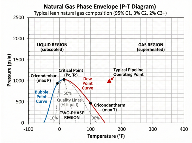
A phase envelope (P-T diagram) shows the pressure-temperature conditions at which a hydrocarbon mixture exists as single-phase gas, single-phase liquid, or two-phase gas-liquid. Understanding phase envelopes is critical for pipeline hydraulics, separator design, gas processing, and avoiding liquid dropout in transmission systems.
Figure 1: Typical natural gas phase envelope showing key features and phase regions.
Phase regions
Gas, liquid, two-phase
Inside envelope: two phases. Outside: single phase (gas at high T/low P; liquid at low T/high P).
Bubble point curve
Left side of envelope
100% liquid at this P/T; any pressure reduction causes first bubble of gas to form.
Dew point curve
Right side of envelope
100% gas at this P/T; any pressure increase or cooling causes first drop of liquid.
Phase Envelope Terminology:
1. Critical Point (P_c, T_c):
- Pressure and temperature where liquid-vapor distinction vanishes
- Where bubble point and dew point curves meet
- For pure components: coincides with cricondenbar (max P)
- For mixtures: typically at lower P than cricondenbar and lower T than cricondentherm
- For pure methane: P_c = 667.8 psia, T_c = -116.6°F
2. Cricondentherm (T_cdt):
- Maximum temperature at which two phases can coexist
- Rightmost point on phase envelope
- Above T_cdt: fluid is always single-phase gas regardless of pressure
- Typical gas condensate: T_cdt = 150-250°F
3. Cricondenbar (P_cdb):
- Maximum pressure at which two phases can coexist
- Topmost point on phase envelope
- For pure components: same as critical point; for mixtures: above P_c
- Above P_cdb: fluid is always single-phase (dense phase)
- Typical gas condensate: P_cdb = 3000-5000 psia
4. Bubble Point Curve:
- Left boundary of two-phase region
- At pressures below bubble point: liquid + gas exist
- All liquid to the left (high P side) of this curve
5. Dew Point Curve:
- Right boundary of two-phase region
- At pressures below dew point: liquid condenses from gas
- All gas to the right (high T side) of this curve
6. Retrograde Region:
- Area between critical point and cricondentherm on dew point side
- Unusual behavior: pressure DROP causes condensation (opposite of normal)
- Critical for gas condensate reservoirs and rich gas pipelines
Typical Phase Envelopes by Fluid Type
Fluid Type
Critical Temp (°F)
Cricondentherm (°F)
Envelope Shape
Behavior
Dry gas (95%+ methane)
-100 to -80
-50 to 0
Narrow, low temperature
Always gas at surface conditions; no liquid dropout
Wet gas (80-90% methane)
-50 to 0
50 to 100
Wider, moderate T
Gas at reservoir, may condense at surface (NGL recovery)
Gas condensate (60-80% C1)
50 to 150
150 to 250
Wide, high T; large retrograde
Gas at reservoir T; retrograde condensation as P drops
Volatile oil (30-50% C1)
200 to 400
300 to 500
Very wide, very high T
Liquid at reservoir, significant gas liberation at surface
Black oil (< 30% C1)
500 to 700
600 to 800
Extremely wide
Liquid in reservoir and at surface; minimal gas release
Impact on Midstream Operations
Pipeline design: Operating line (P-T trajectory along pipeline due to pressure drop and heat transfer) must stay outside phase envelope to prevent liquid dropout. If line crosses into envelope, slug catchers or phase separators required.
Separator design: Separator operating point must be inside two-phase region to achieve gas-liquid separation. Multi-stage separation follows iso-composition lines (vertical drops in P-T space if isothermal).
Compression: Compressor discharge temperature can exceed cricondentherm, causing single-phase gas. Subsequent cooling may cause retrograde condensation, requiring knockout drums.
NGL recovery: Phase envelope determines minimum temperature for NGL extraction. Cryogenic plants cool gas below hydrocarbon dew point to condense C2+ components.
Why phase envelopes matter: A transmission pipeline designed for dry gas (envelope far below operating conditions) will fail if fed gas condensate (envelope extends above operating line). Liquid dropout causes slug flow, erosion, corrosion, and reduced capacity. Example: 36-inch pipeline designed for 1000 psia, 80°F. If gas changes from dry (T_cdt = 0°F) to condensate (T_cdt = 200°F), the operating point (1000 psia, 80°F) moves from outside envelope (safe) to inside envelope (two-phase flow), reducing capacity by 30-50% and causing operational problems. Always verify phase envelope for actual gas composition, not assumed dry gas properties.
2. Critical Point & Key Features
The critical point represents the highest pressure and temperature at which distinct liquid and gas phases can coexist. Above the critical point, the fluid is supercritical — exhibiting properties of both gas (compressibility) and liquid (density). Understanding critical properties is essential for high-pressure pipeline design and supercritical fluid processing.
Critical Point Definition
Critical Properties:
At the critical point:
∂P/∂V = 0 (first derivative)
∂²P/∂²V = 0 (second derivative)
These conditions define the inflection point on P-V isotherm at T_c.
For pure components, critical properties are tabulated (GPA 2145):
Methane: T_c = -116.6°F (190.6 K), P_c = 667.8 psia (46.0 bar)
Ethane: T_c = 90.1°F (305.4 K), P_c = 707.8 psia (48.8 bar)
Propane: T_c = 206.0°F (369.8 K), P_c = 616.3 psia (42.5 bar)
n-Butane: T_c = 305.7°F (425.1 K), P_c = 550.7 psia (38.0 bar)
For mixtures, pseudo-critical properties from mixing rules:
T_c,mix = Σ (y_i × T_c,i) (Kay's Rule - simple mixing)
P_c,mix = Σ (y_i × P_c,i)
Where y_i = mole fraction of component i
More accurate: Use EOS (Peng-Robinson, SRK) to calculate true critical point of mixture by finding locus where (∂P/∂V)_T = 0.
Pseudo-Critical Properties Calculation
Example: Pseudo-Critical for Gas Condensate Mixture
Composition:
C1 (methane): 70 mol%
C2 (ethane): 10 mol%
C3 (propane): 8 mol%
i-C4: 3 mol%
n-C4: 3 mol%
C5+: 6 mol%
Using Kay's Rule:
T_c,mix = 0.70×(-116.6) + 0.10×90.1 + 0.08×206.0 + 0.03×275 + 0.03×305.6 + 0.06×450
T_c,mix = -81.6 + 9.0 + 16.5 + 8.3 + 9.2 + 27.0
T_c,mix = -11.6°F (convert to Rankine: 448.1°R)
P_c,mix = 0.70×667.8 + 0.10×707.8 + 0.08×616.3 + 0.03×529 + 0.03×551 + 0.06×400
P_c,mix = 467.5 + 70.8 + 49.3 + 15.9 + 16.5 + 24.0
P_c,mix = 644 psia
This mixture has critical point approximately at 644 psia, -12°F.
For more accurate phase envelope, use EOS in simulator (HYSYS, Aspen, ProMax) to calculate true critical point and full P-T envelope.
Reduced Properties and Corresponding States
Reduced Pressure and Temperature:
P_r = P / P_c (reduced pressure)
T_r = T / T_c (reduced temperature, absolute scale)
Where:
P = Operating pressure
T = Operating temperature (absolute, °R or K)
P_c, T_c = Critical pressure and temperature
Corresponding states principle:
Fluids at same P_r and T_r exhibit similar behavior (Z-factor, enthalpy, etc.)
This allows generalized correlations for compressibility factor, fugacity, etc.
Standing-Katz chart: Z = f(P_r, T_r)
Lee-Kesler correlation: Uses P_r, T_r, and acentric factor ω
Example:
Gas at 1000 psia, 100°F
P_c,mix = 644 psia, T_c,mix = 448.1°R (from previous example)
T_operating = 100 + 459.67 = 559.67°R
P_r = 1000 / 644 = 1.55
T_r = 559.67 / 448.1 = 1.25
From Standing-Katz chart at P_r = 1.55, T_r = 1.25:
Z ≈ 0.82
This Z-factor used in gas density and flow calculations.
Supercritical Behavior
Region
P vs P_c
T vs T_c
Behavior
Subcritical gas
P < P_c
T > T_c
Cannot be liquefied by compression alone; must cool below T_c first
Subcritical liquid
P > P_c
T < T_c
Cannot be vaporized by heating alone; must reduce P below P_c first
Supercritical fluid
P > P_c
T > T_c
No distinct liquid/gas phases; continuous transition between liquid-like and gas-like density
Near-critical region
0.9 < P_r < 1.1
0.9 < T_r < 1.1
Large property changes with small P/T changes; difficult to model; avoid in process design
Cricondentherm and Cricondenbar Significance
Cricondentherm (T_cdt): Defines maximum operating temperature for pipeline to avoid single-phase gas. If pipeline temperature exceeds T_cdt, fluid remains single-phase gas even at high pressure — important for dense-phase CO₂ pipelines and rich gas transmission.
Cricondenbar (P_cdb): Defines maximum pressure for two-phase region. In high-pressure gas reservoirs (P > P_cdb), fluid may be single-phase liquid even though composition is gas-like. Depressurization causes gas breakout (undersaturated oil behavior).
Distance from critical point: The farther reservoir or pipeline conditions are from the critical point, the easier the phase behavior to predict and control. Near-critical fluids (P_r ≈ 1, T_r ≈ 1) exhibit extreme sensitivity to pressure/temperature changes and require rigorous EOS modeling.
Critical point vs cricondenbar vs cricondentherm: These are three distinct points on the phase envelope of a mixture. The critical point is where bubble and dew curves meet (liquid and vapor become identical). The cricondenbar is the maximum pressure point (top of envelope) — at higher pressure than the critical point for mixtures. The cricondentherm is the maximum temperature point (rightmost on envelope). For dry gas, all three are close together. For gas condensate, they are far apart — T_cdt can be 100-200°F higher than T_c, and P_cdb can be 200-1500 psi higher than P_c. This wide separation creates a large retrograde condensation region. Always distinguish between these points; confusing them leads to incorrect pipeline or process design.
3. Retrograde Condensation Phenomenon
Retrograde condensation is counter-intuitive behavior where reducing pressure causes liquid to condense from a gas, or increasing temperature causes liquid to vaporize. This occurs in the retrograde region between the critical point and cricondentherm. Understanding retrograde behavior is critical for gas condensate reservoir management and rich gas pipeline design.
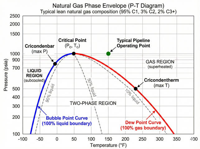
Figure 2: Phase envelope illustrating the retrograde region where pressure reduction causes liquid condensation.
Retrograde Behavior Explained
Retrograde Condensation Process:
Normal behavior (left side of envelope - bubble point):
Pressure decrease: Liquid → Gas (boiling, expected)
Temperature increase: Liquid → Gas (evaporation, expected)
Retrograde behavior (right side of envelope - dew point, between T_c and T_cdt):
Pressure decrease: Gas → Liquid (condensation, counter-intuitive!)
Temperature increase: Liquid → Gas (revaporization, expected)
Why this happens:
In retrograde region, gas is supersaturated with heavy components. As pressure drops:
1. Normally, gas expansion would keep everything gaseous
2. BUT, the heavy components become less soluble in the lighter gas phase
3. Heavy components condense out as liquid (retrograde condensation)
4. Further pressure drop eventually revaporizes the liquid (normal behavior resumes)
Maximum liquid dropout:
Occurs at pressure of maximum liquid formation (typically 1500-2500 psia for gas condensates)
Maximum retrograde condensate: 5-20% liquid by volume (varies with composition)
Temperature effect:
Increasing T in retrograde region causes liquid to revaporize (normal behavior)
This is why heating rich gas pipelines can prevent liquid dropout
Gas Condensate Reservoir Example
Retrograde Liquid Dropout in Reservoir Depletion:
Initial reservoir conditions:
P_initial = 4500 psia
T_reservoir = 250°F (constant)
Gas composition: C1 = 75%, C2-C5 = 20%, C6+ = 5%
Phase envelope:
T_c = 180°F, P_c = 3800 psia
T_cdt = 280°F, P_cdb = 4200 psia
Initial state (4500 psia, 250°F):
Above P_cdb → Single-phase gas (actually near-critical fluid)
As reservoir depletes to 3500 psia (still at 250°F):
Now inside envelope (below dew point curve)
Liquid condenses in reservoir: 8% liquid by volume
This liquid is LOST — cannot be produced (remains in pore space)
Condensate banking around wellbore reduces gas permeability
Further depletion to 2000 psia:
Maximum retrograde liquid: 12% liquid
Further reduction to 1000 psia:
Liquid revaporizes to 5% liquid (retrograde revaporization)
At abandonment (500 psia):
Back to single-phase gas, but 5-15% of reserves left as liquid in reservoir
Mitigation strategies:
1. Gas cycling (inject dry gas to maintain P > dew point)
2. Hydraulic fracturing (bypass condensate bank)
3. Horizontal wells (increase contact area, reduce drawdown)
4. Accept loss (economic if gas price high, condensate value low)
Pipeline Retrograde Condensation
Rich gas pipelines can experience retrograde condensation as pressure drops along the line:
Pipeline Example:
Pipeline inlet: 1200 psia, 100°F (single-phase gas, above dew point)
Pipeline outlet: 800 psia, 100°F (inside envelope, two-phase)
As gas flows and pressure drops:
- At 1100 psia: crosses dew point, liquid begins to condense
- At 1000 psia: 2% liquid by volume
- At 900 psia: 5% liquid (maximum)
- At 800 psia: 4% liquid (starting to revaporize)
Problems:
1. Liquid accumulates at low points (requires pigging or slug catchers)
2. Two-phase flow increases pressure drop (larger compressors needed)
3. Liquid causes corrosion if sour gas (H₂S dissolves in liquid)
4. Hydrates can form in liquid phase at low temperature
Solutions:
1. Heat pipeline to raise T above T_cdt (expensive: insulation, heat tracing)
2. Install separators mid-line to remove liquid (adds cost, complexity)
3. Inject lighter gas to shift phase envelope (if available)
4. Increase line pressure to stay above dew point (larger/more compressors)
5. Accept two-phase flow and design accordingly (slug catchers, pigging, larger diameter)
Retrograde liquid composition: Retrograde condensate is much richer in heavy components (C5+) than the original gas. While gas may be 75% C1, the retrograde liquid can be 60-80% C5+ (C5-C12 range). This makes retrograde condensate valuable (high API gravity, 50-60° API, worth more than crude oil) but also problematic (high vapor pressure, requires stabilization before sales). In gas condensate fields, this retrograde liquid trapped in the reservoir represents significant lost revenue — motivating gas cycling or pressure maintenance projects to keep reservoir pressure above the dew point.
4. Hydrate Formation Curves
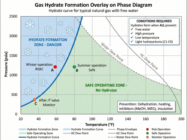
Gas hydrates are ice-like crystalline solids formed when water and light hydrocarbons (C1-C4) combine under high pressure and low temperature. Hydrates can plug pipelines, valves, and equipment, causing safety hazards and production shutdowns. Hydrate formation curves overlay on phase envelopes to show conditions where hydrates are thermodynamically stable.
Figure 3: Hydrate formation curve overlaid on phase diagram showing safe vs. danger zones for pipeline operations.
Hydrate Formation Conditions
Hydrate Stability Zone:
Hydrates form when ALL three conditions are met:
1. Free water present (liquid water or ice)
2. Pressure above hydrate formation pressure at given temperature
3. Temperature below hydrate formation temperature at given pressure
4. Light hydrocarbons present (C1, C2, C3, i-C4; n-C4 barely forms hydrates; C5+ do not)
Hydrate formation curve:
Plots P vs T boundary where hydrates become stable
Approximately exponential: hydrate pressure increases rapidly with temperature
For natural gas, use Katz gas gravity chart (GPSA Fig. 20-11):
- Plot gas gravity (0.55-1.0) vs temperature to read formation pressure
- Heavier gas (higher gravity) → hydrates form at lower pressure (more prone)
- Lighter gas (lower gravity) → hydrates form at higher pressure (less prone)
For detailed predictions:
- Katz K-value method (moderate accuracy, hand calculation)
- CSMGem, Multiflash, PVTsim software (high accuracy, includes inhibitors)
- PIPESIM, OLGA for transient hydrate modeling in pipelines
Typical hydrate formation:
At 32°F (ice point): Hydrates form at ~200-300 psia for natural gas
At 50°F: Hydrates form at ~600-800 psia
At 70°F: Hydrates form at ~2000-3000 psia
Higher pressure → higher hydrate formation temperature
Heavier gas (more C2, C3) → higher hydrate formation temperature (worse)
Hydrate Structures
Structure
Guest Molecules
Cage Type
Typical Gas
Structure I (sI)
Small molecules (CH₄, C₂H₆, CO₂, H₂S)
12-sided, 14-sided cavities
Dry natural gas, lean gas
Structure II (sII)
Larger molecules (C₃H₈, i-C₄H₁₀)
12-sided, 16-sided cavities
Rich gas with propane/butane
Structure H (sH)
Very large molecules (C₅+, cyclopentane)
12-sided, 20-sided cavities
Gas with heavy hydrocarbons (rare in midstream)
Hydrate Prevention Methods
Thermodynamic Inhibition (Shift Hydrate Curve to Left):
1. Methanol (MeOH) injection:
Depresses hydrate formation temperature
Dosage: 15-35 wt% in water phase
Hammerschmidt Equation (GPSA):
ΔT = K_H × W / (M × (100 - W))
Solving for required concentration:
W = 100 × M × ΔT / (K_H + M × ΔT)
Where:
ΔT = desired hydrate depression (°F)
K_H = 2335 (Hammerschmidt constant for °F units)
M = molecular weight of inhibitor (32.04 for MeOH)
W = wt% inhibitor in aqueous phase
Example:
Need 20°F depression:
W = 100 × 32.04 × 20 / (2335 + 32.04 × 20)
W = 64,080 / 2,976 = 21.5 wt% MeOH
2. Monoethylene Glycol (MEG) injection:
Similar to MeOH but less volatile (preferred for high-pressure systems)
Dosage: 20-50 wt% in water phase
More expensive than MeOH but can be regenerated and reused
3. Kinetic Hydrate Inhibitors (KHI):
Low-dosage polymers (0.5-3 wt%) that delay hydrate nucleation
Do not shift hydrate curve; allow subcooling of 10-20°F
Cheaper than MeOH/MEG but limited to moderate subcooling
Examples: PVCap (polyvinylcaprolactam), VC-713
4. Anti-Agglomerants (AA):
Surfactants that prevent hydrate crystals from agglomerating into plugs
Allow hydrates to form but keep them dispersed in liquid
Dosage: 0.5-2 wt%
Effective for high water cuts; require continuous liquid phase
Hydrate Formation Curve Overlay on Phase Envelope
Combined P-T Diagram:
On phase envelope diagram, also plot:
1. Hydrocarbon dew point curve (phase envelope)
2. Water dew point curve (100% RH line)
3. Hydrate formation curve
Critical zones:
Zone 1: Above hydrocarbon dew point, above water dew point
→ Single-phase gas, no free water → NO HYDRATES (safe)
Zone 2: Below hydrocarbon dew point, above water dew point
→ Two-phase hydrocarbons, no free water → NO HYDRATES (safe if no water)
Zone 3: Above hydrocarbon dew point, below water dew point, above hydrate curve
→ Gas + liquid water present → HIGH HYDRATE RISK
Zone 4: Inside hydrate zone
→ Hydrates thermodynamically stable → WILL FORM if water present
Typical pipeline scenario:
Inlet: 1000 psia, 80°F (above all curves - safe)
Outlet: 600 psia, 60°F (inside hydrate zone if water present)
→ Must dehydrate gas OR inject inhibitor OR heat pipeline
Water dewpoint of natural gas:
Depends on pressure and water content (lb H₂O / MMscf)
Pipeline spec: < 7 lb/MMscf (very dry gas; water dew point < -20°F)
Wet gas from wellhead: 200-2000 lb/MMscf (water dew point 60-100°F)
Hydrate Plug Remediation
Depressurization: Reduce pressure below hydrate formation curve. Slow process (hours to days) but effective. Risk: hydrate dissociation releases large volume of gas (1 ft³ hydrate → 160 ft³ gas); can cause pressure surge.
Heating: Apply external heat (hot water, steam, electrical heating) to raise temperature above hydrate curve. Faster than depressurization but expensive and difficult in long pipelines.
Inhibitor injection: Pump MeOH or MEG into plug location. Slow diffusion into plug (can take days). Requires access point upstream and downstream of plug.
Pigging: If plug is soft, pig can push it out. Risk: hard plug can jam pig and make situation worse. Never pig a suspected hydrate plug without confirmation of plug location and hardness.
Hydrate prevention is cheaper than remediation: Removing a hydrate plug from a 24-inch pipeline can cost $500K-$5M in lost production, equipment rental (coiled tubing, hot oil pumps), and labor. Annual MeOH injection costs $50-200K. Dehydration (TEG or mol sieve) costs $2-5M CAPEX but eliminates hydrate risk permanently and avoids ongoing inhibitor costs. For new pipelines, always specify dehydration to < 7 lb/MMscf (pipeline quality) to avoid hydrate issues. For existing systems with hydrate history, conduct detailed hydrate curve analysis and implement reliable inhibition program with redundancy (backup injection pumps, MeOH storage for 30+ days).
5. Equation of State Modeling
Cubic equations of state (EOS) like Peng-Robinson (PR) and Soave-Redlich-Kwong (SRK) are the industry standard for predicting phase behavior of hydrocarbon mixtures. EOS models calculate phase envelopes, flash calculations, density, enthalpy, and fugacity from composition, pressure, and temperature. Modern process simulators (Aspen, HYSYS, ProMax) use EOS for all thermodynamic property predictions.
Figure 4: Phase envelope comparison showing how composition affects envelope size - heavier fluids have larger envelopes.
Peng-Robinson Equation of State
Peng-Robinson EOS (1976):
P = RT/(V-b) - a·α(T) / [V(V+b) + b(V-b)]
Where:
P = Pressure
V = Molar volume
T = Absolute temperature
R = Universal gas constant
Component parameters:
a = 0.45724 × R² × T_c² / P_c
b = 0.07780 × R × T_c / P_c
Temperature function:
α(T) = [1 + κ(1 - √(T/T_c))]²
Where:
κ = 0.37464 + 1.54226ω - 0.26992ω²
ω = Acentric factor (measure of molecular non-sphericity)
For mixtures, use mixing rules:
a_mix = Σ Σ (x_i × x_j × √(a_i × a_j) × (1 - k_ij))
b_mix = Σ (x_i × b_i)
Where:
x_i = Mole fraction of component i
k_ij = Binary interaction parameter (adjusts for unlike-molecule interactions)
Advantages of PR-EOS:
- Accurate for gas and liquid density (±1-5%)
- Good for vapor-liquid equilibrium (VLE) calculations
- Widely used in oil/gas industry (20+ years of validation)
- Reliable for hydrocarbons from C1 to C20+
Limitations:
- Less accurate near critical point (±10-20% error)
- Polar components (water, alcohols) require special treatment
- Binary interaction parameters needed for accuracy (fitted to data)
Soave-Redlich-Kwong Equation of State
SRK EOS (1972):
P = RT/(V-b) - a·α(T) / [V(V+b)]
Similar form to PR but simpler denominator in attractive term.
Component parameters:
a = 0.42748 × R² × T_c² / P_c
b = 0.08664 × R × T_c / P_c
Temperature function (same as PR):
α(T) = [1 + κ(1 - √(T/T_c))]²
κ = 0.480 + 1.574ω - 0.176ω²
Differences vs Peng-Robinson:
- SRK slightly less accurate for liquid density
- SRK better for high-pressure gas systems (> 5000 psia)
- PR better for NGL and LPG applications
- Both give similar results for most natural gas applications
Industry practice:
- Use PR for general oil/gas, NGL, LPG
- Use SRK for high-pressure gas reservoirs, gas injection
- Use specialized EOS (GERG-2008, AGA-8) for custody transfer
Flash Calculation (Phase Split)
Rachford-Rice Flash Equation:
Given: Overall composition z_i, Pressure P, Temperature T
Find: Vapor fraction β, vapor composition y_i, liquid composition x_i
Equilibrium relation:
y_i = K_i × x_i
Where K_i = vapor-liquid equilibrium ratio (K-value)
Material balance:
z_i = β × y_i + (1-β) × x_i
Combining:
z_i = β × K_i × x_i + (1-β) × x_i
z_i = x_i × [β × K_i + (1-β)]
x_i = z_i / [1 + β × (K_i - 1)]
y_i = K_i × z_i / [1 + β × (K_i - 1)]
Rachford-Rice objective function:
f(β) = Σ [z_i × (K_i - 1) / (1 + β × (K_i - 1))] = 0
Solve for β using Newton-Raphson iteration.
K-values from EOS:
K_i = φ_i^L / φ_i^V
Where φ = fugacity coefficient (calculated from EOS)
Process:
1. Guess β (start with 0.5)
2. Calculate K_i from EOS at P, T
3. Solve Rachford-Rice for new β
4. Update K_i based on new x_i, y_i compositions
5. Iterate until convergence (β changes < 0.001)
Results:
- If β = 0: All liquid (below bubble point)
- If 0 < β < 1: Two-phase (inside envelope)
- If β = 1: All vapor (above dew point)
What this calculator actually uses: A rigorous Peng-Robinson fugacity flash (Ki = φiL/φiV, iterated as above) is the high-accuracy reference shown for completeness. This screening tool instead estimates the bubble and dew points from the Wilson correlation for K-values:
The Wilson correlation needs only each component's critical pressure, critical temperature, and acentric factor (no EOS iteration), which makes it fast and robust for screening — but it is less accurate than a full PR/SRK flash near the critical point and for heavy, non-ideal mixtures. Use process simulation (PR/SRK with fugacity, the method above) for design-grade work.
Phase Envelope Calculation Procedure
Generating Phase Envelope from EOS:
Bubble point curve (left side):
Starting from low T, increment T and solve for P where first vapor bubble forms.
At each T:
- Assume all liquid (x_i = z_i)
- Calculate K_i from EOS
- Iterate P until Σ(K_i × x_i) = 1.0
- This P is bubble point pressure at T
Dew point curve (right side):
Starting from low T, increment T and solve for P where first liquid drop forms.
At each T:
- Assume all vapor (y_i = z_i)
- Calculate K_i from EOS
- Iterate P until Σ(z_i / K_i) = 1.0
- This P is dew point pressure at T
Critical point:
Find (P, T) where bubble point and dew point curves converge.
Numerically: where ∂P/∂V = 0 and ∂²P/∂²V = 0 from EOS.
Quality lines (constant liquid %):
For each (P, T) inside envelope:
- Perform flash calculation to get β
- Plot line connecting all (P, T) where β = 0.1 (10% vapor = 90% liquid)
- Repeat for β = 0.5, 0.9, etc.
Modern simulators automate this process:
- Aspen HYSYS: Use "Phase Envelope" utility
- ProMax: Use "2-Phase PT" envelope tool
- Multiflash: Specialized for complex phase behavior
Tuning EOS to Match Experimental Data
Binary interaction parameters (k_ij): Adjust k_ij values to match separator test data (GOR, liquid density, bubble point). Typical k_ij for C1-C10 = 0 to 0.15; for C1-H2O = 0.50 (large value due to polarity difference).
C7+ characterization: Split C7+ fraction into pseudo-components (C7-C12, C13-C20, C21-C30, etc.) using distillation data or correlations (Pedersen, Whitson). Use measured density and molecular weight to improve heavy-end predictions.
Shift critical properties: For gas condensates, shift T_c and P_c of C7+ fractions to match critical point from lab PVT study. Typical shifts: ±5-10% to match measured cricondentherm.
Volume shift: Add volume correction (c_i parameter) to PR or SRK to improve liquid density predictions. Standard PR underpredicts liquid density by 5-15%; volume shift corrects this.
EOS accuracy and validation: Untuned EOS (default parameters) can predict phase envelopes with ±10-30% error in critical point and cricondentherm. For critical applications (gas condensate reservoir, retrograde pipeline, cryogenic NGL plant), always validate EOS against experimental PVT data: (1) Constant composition expansion (CCE) to measure dew point, (2) Constant volume depletion (CVD) to measure retrograde liquid dropout, (3) Separator tests to measure GOR and liquid properties. Tuning EOS to match lab data reduces error to ±2-5%, essential for reliable facility design. Cost of PVT study: $15-30K. Cost of undersized separator or pipeline: $1-10M+. Always invest in good PVT data for projects > $10M.
A phase envelope diagram maps the boundary between single-phase and two-phase regions for a gas mixture, showing the bubble point and dew point curves on a pressure-temperature plot.
What are cricondentherm and cricondenbar?+
Cricondentherm is the maximum temperature on the phase envelope above which no liquid forms, and cricondenbar is the maximum pressure above which no vapor-liquid separation occurs.
What is retrograde condensation?+
Retrograde condensation is the phenomenon where liquid forms as pressure decreases below the dew point within the phase envelope, contrary to normal vaporization behavior.
What equations of state are used for phase envelope modeling?+
Peng-Robinson and SRK (Soave-Redlich-Kwong) equations of state are commonly used for phase envelope modeling of natural gas systems.