Calculate gas leak rates through orifices and pipeline ruptures, distinguish choked vs unchoked flow regimes, apply API 581 hole size categories, and perform dispersion modeling for emergency response planning.
Perform quantitative risk assessment (QRA) per API 581.
1. Overview & Applications
Gas leak rate calculations are fundamental to process safety management, risk-based inspection (RBI), emergency response planning, and regulatory compliance. Accurate leak rate prediction enables proper sizing of safety systems, evaluation of hazard zones, and prioritization of integrity management activities.
Quantitative risk assessment
QRA & RBI (API 581)
Consequence modeling requires leak rates for small, medium, large, and rupture scenarios.
Emergency shutdown sizing
ESD valve capacity
ESD systems must isolate inventory faster than critical leak rates.
Dispersion modeling
Flammable cloud extent
PHAST, ALOHA, or CFD models require source leak rate as primary input.
Regulatory compliance
EPA RMP & OSHA PSM
Risk Management Plans require worst-case and alternative release scenarios.
Key Concepts
Choked flow: Sonic velocity at orifice; mass flow rate independent of downstream pressure
Unchoked (subsonic) flow: Mass flow depends on pressure differential across orifice
Critical pressure ratio: P_d/P_u threshold below which flow becomes choked (~0.528 for ideal gas, k=1.4)
Discharge coefficient (Cd): Accounts for real orifice geometry vs idealized sharp-edged hole (typically 0.6-1.0)
Blowdown time: Duration to depressurize vessel or pipe segment after isolation
Why leak rates matter: A 1-inch diameter hole in a 600 psig natural gas pipeline releases approximately 5-8 lb/s (400-600 Mscf/hr) depending on hole geometry. Within 60 seconds, this forms a flammable vapor cloud exceeding 100,000 ft³ at lower flammable limit (LFL). Accurate leak rate prediction is essential for determining safe separation distances and emergency response times.
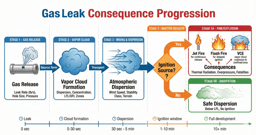
Gas leak consequence progression from initial release through vapor cloud formation to potential fire/explosion or safe dispersion outcomes
2. Orifice Leak Rate Equations
Gas flow through an orifice (leak, hole, or rupture) is governed by compressible flow equations. The mass flow rate depends on upstream pressure, temperature, gas properties, hole size, and whether flow is choked or unchoked.
General Orifice Flow Equation
Mass Flow Rate Through Orifice:
ṁ = Cd × A × ρ × V
Where:
ṁ = Mass flow rate (lb/s or kg/s)
Cd = Discharge coefficient (dimensionless, typically 0.6-1.0)
A = Orifice area (ft² or m²)
ρ = Gas density upstream (lb/ft³ or kg/m³)
V = Gas velocity through orifice (ft/s or m/s)
For compressible flow, velocity and density are coupled through thermodynamics.
Choked Flow (Sonic) Equation
Choked Flow (P_d/P_u ≤ Critical Ratio):
The isentropic choked mass flow rate through an orifice:
ṁ = Cd × A × P₁ × √(g_c × MW / (R_mech × T₁ × Z₁)) × C
Where C = √[ k × (2/(k+1))^((k+1)/(k-1)) ] (choked flow constant)
In practical US customary units (A in in², P in psia, T in °R):
ṁ (lb/s) = Cd × A (in²) × P₁ (psia) × 0.1443 × C × √(MW / (T₁(°R) × Z₁))
The combined coefficient (0.1443 × C) varies with k:
k = 1.27 (natural gas): 0.1443 × 0.662 = 0.0955
k = 1.30 (methane): 0.1443 × 0.667 = 0.0963
k = 1.40 (air): 0.1443 × 0.685 = 0.0988
Where:
0.1443 = √(g_c / R_mech) = √(32.174 / 1545.35)
g_c = 32.174 lbm·ft/(lbf·s²) (gravitational conversion constant)
R_mech = 1545.35 ft·lbf/(lbmol·°R) (universal gas constant)
k = Specific heat ratio (Cp/Cv, typically 1.27-1.40 for natural gas)
MW = Molecular weight (lb/lbmol)
T₁ = Upstream temperature (°R = °F + 459.67)
Z₁ = Compressibility factor at upstream conditions
P₁ = Upstream absolute pressure (psia)
Critical pressure ratio (choked flow threshold):
P_crit/P₁ = (2/(k+1))^(k/(k-1))
For k = 1.4: P_crit/P₁ = 0.528
If P_downstream < 0.528 × P_upstream, flow is choked.
Unchoked Flow (Subsonic) Equation
Unchoked Flow (P_d/P_u > Critical Ratio):
ṁ = Cd × A × P₁ × 0.1443 × √[(2k/(k-1)) × (MW/(T₁×Z₁)) × ((P₂/P₁)^(2/k) - (P₂/P₁)^((k+1)/k))]
Where:
P₂ = Downstream absolute pressure (psia)
0.1443 = √(g_c / R_mech) (same constant as choked equation)
The expansion term [(P₂/P₁)^(2/k) - (P₂/P₁)^((k+1)/k)] replaces the
choked flow constant C, and captures the pressure-ratio dependence.
For small pressure drops (P₂/P₁ > 0.8), unchoked flow can be approximated:
ṁ ≈ Cd × A × √(2 × ρ₁ × ΔP) (incompressible approximation)
Worked Example: Choked Flow
Calculate mass flow rate through a 1-inch diameter hole in a natural gas pipeline at 800 psig, 80°F:
Given:
Hole diameter d = 1.0 inch
Upstream pressure P₁ = 800 + 14.7 = 814.7 psia
Upstream temperature T₁ = 80 + 459.67 = 539.67 °R
Gas properties: MW = 18.0, k = 1.27, Z₁ = 0.92
Discharge coefficient Cd = 0.85 (rounded/short-tube hole)
Downstream pressure P₂ = 14.7 psia (atmospheric)
Step 1: Check if flow is choked
Critical ratio = (2/(k+1))^(k/(k-1))
For k = 1.27: Critical ratio = (2/2.27)^(1.27/0.27) = 0.551
P₂/P₁ = 14.7 / 814.7 = 0.018 << 0.551
Flow IS choked (sonic at orifice throat).
Step 2: Calculate orifice area
A = π × d² / 4 = π × 1.0² / 4 = 0.785 in²
Step 3: Calculate choked flow constant C
C = √[ k × (2/(k+1))^((k+1)/(k-1)) ]
C = √[ 1.27 × (2/2.27)^(2.27/0.27) ]
C = √[ 1.27 × 0.345 ] = √0.438 = 0.662
Combined coefficient = 0.1443 × 0.662 = 0.0955
Step 4: Apply choked flow equation
ṁ = Cd × A × P₁ × 0.0955 × √(MW / (T₁ × Z₁))
ṁ = 0.85 × 0.785 × 814.7 × 0.0955 × √(18.0 / (539.67 × 0.92))
ṁ = 0.85 × 0.785 × 814.7 × 0.0955 × √(0.0363)
ṁ = 0.85 × 0.785 × 814.7 × 0.0955 × 0.1904
ṁ = 9.89 lb/s
Step 5: Convert to volumetric flow at standard conditions
For 1 lbmol ideal gas at 14.7 psia, 60°F: V = 379.5 scf/lbmol
Mass per mole = 18.0 lb/lbmol
scf/hr = (9.89 lb/s × 3600 s/hr) / (18.0 lb/lbmol) × 379.5 scf/lbmol
scf/hr = 750,600 scf/hr = 750.6 Mscf/hr = 18,014 Mscfd
Result:
A 1-inch hole at 800 psig releases 9.9 lb/s or 18,000 Mscfd of natural gas.
In 1 minute: 593 lb or 12,500 scf released
In 10 minutes: 5,934 lb or 125,100 scf released
Note: This is the instantaneous rate at full upstream pressure.
In practice, pipeline pressure decays after isolation, reducing the leak rate over time.
Discharge Coefficient (Cd) Values
Orifice Type
Typical Cd
Description
Sharp-edged circular hole
0.60-0.65
Corrosion pit, drilled hole, puncture
Well-rounded nozzle
0.95-1.00
Machined opening, flange connection
Short pipe (L/d = 2-3)
0.80-0.85
Crack with depth, weld defect
Long pipe (L/d > 10)
0.70-0.75
Through-wall crack, corroded pathway
Rupture (guillotine break)
1.00
Full-bore pipe rupture (no orifice restriction)
Safety valve discharge
0.975 (per ASME)
Certified relief valve orifice
Conservative practice: For leak rate safety studies, use Cd = 1.0 to predict maximum (worst-case) release rate. For realistic consequence modeling, use Cd = 0.6-0.85 based on expected hole morphology.
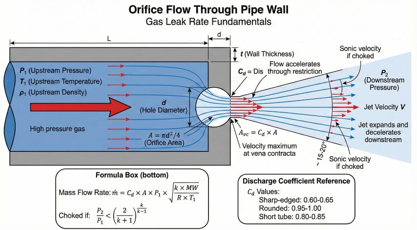
Orifice flow through pipe wall showing upstream conditions, vena contracta formation, and downstream jet expansion with discharge coefficient reference
3. Choked vs Unchoked Flow Regimes
Understanding whether gas flow is choked (sonic) or unchoked (subsonic) is critical for accurate leak rate prediction. Choked flow is independent of downstream pressure, simplifying calculations for atmospheric releases.
Flow Regime Determination
Critical Pressure Ratio as Function of k:
P_crit / P_upstream = (2 / (k+1))^(k/(k-1))
k value Critical ratio Application
1.40 0.528 Air, nitrogen, oxygen
1.30 0.546 Methane (approx)
1.27 0.551 Natural gas (typical)
1.20 0.565 Ethane, heavier gases
1.10 0.585 CO₂, refrigerants
Decision rule:
IF (P_downstream / P_upstream) < Critical_ratio THEN
Flow is CHOKED (use choked equation)
ELSE
Flow is UNCHOKED (use subsonic equation)
END IF
Example:
Natural gas (k = 1.27) at 600 psig = 614.7 psia
Discharging to atmosphere (14.7 psia)
P_d / P_u = 14.7 / 614.7 = 0.024 < 0.551 → CHOKED
Same gas discharging to downstream vessel at 400 psia:
P_d / P_u = 400 / 614.7 = 0.651 > 0.551 → UNCHOKED
Velocity at Choked Conditions
Sonic Velocity (Speed of Sound in Gas):
a = √(k × R × T / MW)
In US units:
a (ft/s) = 223.0 × √(k × T(°R) / MW)
Where 223.0 = √(g_c × R_mech) = √(32.174 × 1545.35)
For natural gas (MW = 18, k = 1.27) at 80°F (540°R):
a = 223.0 × √(1.27 × 540 / 18)
a = 223.0 × √(38.1)
a = 223.0 × 6.17
a = 1,376 ft/s = 939 mph
This is the maximum exit velocity for choked flow.
Density and velocity at throat (choked conditions):
At sonic throat, Mach number M = 1.0
ρ_throat = ρ_upstream × (2/(k+1))^(1/(k-1))
V_throat = a (speed of sound)
For k = 1.27:
ρ_throat = 0.626 × ρ_upstream
Significant density reduction due to isentropic expansion.
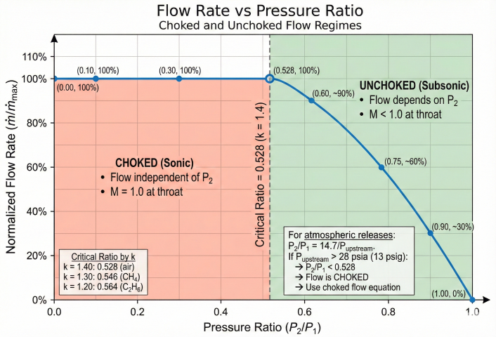
Effect of Downstream Pressure on Flow Rate
For unchoked flow, mass flow rate increases as pressure differential increases:
P_d/P_u Ratio
Flow Regime
ṁ / ṁ_choked
Notes
1.00
No flow
0%
No pressure differential
0.90
Unchoked
~30%
Small ΔP, low flow
0.75
Unchoked
~60%
Moderate ΔP
0.60
Near choked
~90%
Approaching sonic conditions
0.528 (k=1.4)
Critical
100%
Transition to choked flow
< 0.528
Choked
100%
Flow rate independent of P_d
Normalized flow rate versus pressure ratio showing transition between choked and unchoked flow regimes at critical pressure ratio
Practical Implications for Safety Studies
Atmospheric releases: Nearly all high-pressure gas releases to atmosphere are choked (P_u > 30 psia typically); use choked equation
Releases into confined spaces: Downstream pressure can build up, potentially transitioning from choked to unchoked; requires dynamic modeling
Isolation valve closure: As upstream pressure decays after isolation, flow may transition from choked to unchoked before stopping
Conservative assumption: Always assume choked flow for maximum leak rate unless proven otherwise by pressure ratio calculation
Blowdown Time Estimation
Vessel Blowdown Through Orifice (Choked Flow):
For isothermal blowdown (constant temperature assumption), the choked flow rate
is proportional to pressure: ṁ(P) ∝ P. This gives exponential pressure decay:
dP/dt = −λ × P → P(t) = P₁ × e^(−λt)
Where λ = Cd × A_ft² × 0.1443 × C × √(MW/(T×Z)) × R_mech × T × Z / (V × MW)
Solving for time to reach P₂:
t = (1/λ) × ln(P₁ / P₂)
Example: 1000 ft³ vessel at 500 psia, 1-inch orifice, blow to 50 psia
A = π × (1/12)² / 4 = 0.00545 ft²
C = √[1.27 × (2/2.27)^(2.27/0.27)] = 0.662
Cd = 0.85, MW = 18.0, T = 540 °R, Z = 0.92
λ = 0.85 × 0.00545 × 0.1443 × 0.662 × √(18/(540×0.92)) × 1545.35 × 540 × 0.92 / (1000 × 18)
λ = 0.003594 /s
t = (1/0.003594) × ln(500/50)
t = 278.3 × 2.303
t = 641 seconds ≈ 10.7 minutes
Key insight: Even a 1-inch orifice can depressurize a 1000 ft³ vessel from
500 to 50 psia in about 11 minutes. However, for a long pipeline segment (miles of
pipe with much larger volume), blowdown through a small leak can take hours.
For emergency depressuring, API 521 recommends sizing depressuring valves to reduce
pressure to 50% within 15 minutes (fire case).
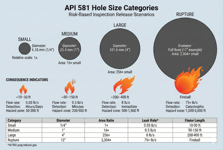
4. API 581 Hole Size Categories
API Recommended Practice 581 (Risk-Based Inspection Methodology) defines four standardized hole size categories for consequence analysis. These categories represent small leaks, medium leaks, large leaks, and full-bore ruptures, each with different safety and environmental consequences.
API 581 standardized hole size categories for risk-based inspection consequence analysis with relative scale comparison and consequence indicators
API 581 Hole Size Definitions
Category
Hole Diameter
Typical Causes
Detection
Small
6.35 mm (0.25 inch, 1/4")
Pinhole corrosion, small crack, threaded connection leak
Often undetected for hours/days; may be found by gas detector or inspection
Jet flame 200-400 ft; major fire, thermal radiation hazard
Rupture (full bore)
1,000-3,000 ft radius
Very large area (> 300m)
Fireball or large jet flame; severe damage, fatalities likely
Frequency Assumptions (API 581 Generic)
API 581 provides generic failure frequencies for uninspected equipment:
Typical failure frequencies (events per year per pipe segment):
Small hole: 1 × 10⁻⁴ to 1 × 10⁻³ (1 in 10,000 to 1 in 1,000 per year)
Medium hole: 1 × 10⁻⁵ to 1 × 10⁻⁴ (1 in 100,000 to 1 in 10,000 per year)
Large hole: 1 × 10⁻⁶ to 1 × 10⁻⁵ (1 in 1,000,000 to 1 in 100,000 per year)
Rupture: 1 × 10⁻⁷ to 1 × 10⁻⁶ (1 in 10,000,000 to 1 in 1,000,000 per year)
These are modified by:
- Corrosion rate and inspection effectiveness
- Mechanical damage susceptibility
- Equipment complexity
- Management system quality
- Prior inspection findings
Risk calculation:
Risk = Frequency × Consequence
For medium hole scenario:
Frequency = 5 × 10⁻⁵ per year
Consequence = $500,000 (property damage + business interruption)
Risk = 5 × 10⁻⁵ × $500,000 = $25/year expected loss
Aggregate across all scenarios for total risk per equipment item.
5. Gas Dispersion Modeling & Emergency Response
Leak rate calculations provide the source term for gas dispersion modeling, which predicts downwind concentrations, flammable cloud extent, and toxic exposure zones. This information is critical for emergency planning, facility siting, and public safety.
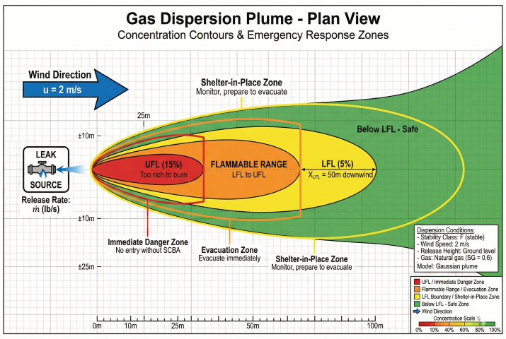
Gas dispersion plume plan view with concentration contours and emergency response zone delineation based on Gaussian dispersion model
Dispersion Modeling Overview
Gaussian plume models
ALOHA, DEGADIS
Simple steady-state plume models for neutral or buoyant gases; regulatory screening.
Dense gas models
PHAST, SLAB
For heavier-than-air gases (propane, CO₂); accounts for gravity slumping.
CFD modeling
FLACS, ANSYS Fluent
High-fidelity 3D models for complex geometry, congestion, and explosion overpressure.
Jet release
PHAST jet model
High-momentum jets from pressurized releases; entrainment and mixing.
Key Dispersion Parameters
Source Term (from leak rate calculation):
Mass flow rate: ṁ (lb/s or kg/s)
Release height: H (m, typically 0-10m for pipeline)
Exit velocity: V_exit (m/s, from choked or unchoked calculation)
Exit temperature: T_exit (K, often cooler due to Joule-Thomson expansion)
Atmospheric conditions:
Wind speed: u (m/s, at 10m height)
Atmospheric stability class: A-F (Pasquill-Gifford)
A, B = Unstable (daytime, strong solar, good mixing)
D = Neutral (overcast or transition)
E, F = Stable (nighttime, calm, poor mixing - worst case)
Temperature: T_amb (K)
Relative humidity: RH%
Gas properties:
Molecular weight: MW
Lower flammable limit: LFL (vol%, e.g., 5% for methane)
Upper flammable limit: UFL (vol%, e.g., 15% for methane)
Toxic limit: IDLH, ERPG-2, etc. (ppm)
Output from dispersion model:
Concentration C(x,y,z,t) as function of position and time
Distance to LFL (flammable cloud extent)
Distance to toxic threshold (IDLH, ERPG-2)
Affected population count (if site-specific census data available)
Flammable Cloud Footprint Estimation
Simplified screening calculation for downwind distance to LFL (natural gas, LFL = 5%):
Rough screening formula (Gaussian plume, ground-level release):
X_LFL ≈ K × (ṁ / (u × C_LFL))^0.5
Where:
X_LFL = Downwind distance to LFL (m)
K = Empirical constant (5-10 depending on stability)
ṁ = Mass release rate (kg/s)
u = Wind speed (m/s)
C_LFL = LFL concentration (kg/m³)
Example: Medium hole (1-inch) releasing 11.3 lb/s = 5.1 kg/s
Natural gas: LFL = 5% by volume
At ambient, 5% methane by volume ≈ 0.04 kg/m³
Wind speed u = 2 m/s (light wind, conservative)
Stability class F (stable, worst case): K ≈ 8
X_LFL ≈ 8 × (5.1 / (2 × 0.04))^0.5
X_LFL ≈ 8 × (63.8)^0.5
X_LFL ≈ 8 × 7.99
X_LFL ≈ 64 meters = 210 feet
For large hole (4-inch, ṁ = 180 lb/s = 81.8 kg/s):
X_LFL ≈ 8 × (81.8 / (2 × 0.04))^0.5 = 8 × 32.0 = 256 meters = 840 feet
Note: This is simplified screening only. Use PHAST, ALOHA, or equivalent
for regulatory submittals. High-pressure jet releases have longer reach due to
momentum, requiring specialized jet dispersion models.
Emergency Response Planning
Leak rate calculations inform emergency shutdown (ESD) system design and response procedures:
Response Element
Small Leak
Medium Leak
Large Leak/Rupture
Detection time
Minutes to hours
Seconds to minutes
Immediate (< 1 sec)
ESD activation
Manual (operator decision)
Automatic (gas detector)
Automatic (pressure/flow anomaly)
Isolation time target
5-15 minutes acceptable
1-3 minutes required
< 30 seconds critical
Evacuation
Localized (equipment area)
Unit evacuation (200-500 ft)
Site evacuation (1,000+ ft)
Emergency services
On-site response sufficient
Fire department standby
Full emergency response (fire, hazmat, EMS)
Inventory at Risk (IAR)
Inventory Between Isolation Valves:
For pipeline segment of length L and diameter D:
V_pipe = π × D² / 4 × L
Mass inventory = V_pipe × ρ
Where ρ is density at line conditions (use real gas density).
Example: 12-inch pipeline, 5 miles between ESD valves
D = 1.0 ft (12-inch ID)
L = 5 miles × 5,280 ft/mile = 26,400 ft
V = π × 1.0² / 4 × 26,400 = 20,740 ft³
At 900 psig, 70°F, natural gas (SG = 0.6, MW = 17.5, Z = 0.89):
ρ = (P × MW) / (Z × R × T)
ρ = (914.7 × 17.5) / (0.89 × 10.73 × 529.67)
ρ = 3.14 lb/ft³
Mass inventory = 20,740 ft³ × 3.14 lb/ft³ = 65,100 lb
Standard volume = 65,100 / 17.5 × 379.5 = 1,412,000 scf = 1.4 MMscf
Blowdown after isolation (12-inch rupture):
Initial release rate = 1,622 lb/s (from API 581 rupture example)
As pressure decays, release rate decreases proportionally:
ṁ(t) ≈ ṁ_initial × (P(t) / P_initial)
Typical blowdown to 10% initial pressure in 30-60 seconds for large rupture.
Total release ≈ 50-70% of inventory before pressure drops below choking threshold.
Expected release = 0.6 × 65,100 lb = 39,000 lb = 17.7 tons
This forms a massive flammable cloud requiring wide evacuation zone.
Regulatory Requirements
EPA Risk Management Plan (RMP - 40 CFR 68): Facilities with threshold quantities of regulated substances must model worst-case and alternative release scenarios
OSHA PSM (29 CFR 1910.119): Process Hazard Analysis (PHA) must identify and quantify potential releases
DOT Pipeline Safety (49 CFR 192): Integrity Management requires consequence modeling for High Consequence Areas (HCA)
State/local regulations: California CUPA, Texas RRC, and other state agencies may have additional modeling requirements
Emergency planning zones: Modern practice establishes graduated response zones based on dispersion modeling: (1) Immediate hazard zone (IDLH or > UFL), (2) Evacuation zone (LFL to UFL or toxic threshold), and (3) Shelter-in-place zone (below LFL/toxic but observable). Leak rate calculations are the foundation for determining these critical distances.
Common Pitfalls
Assuming unchoked flow for atmospheric release: Most high-pressure releases are choked; using unchoked equation underestimates rate by 30-50%
Using Cd = 1.0 for all scenarios: Sharp-edged holes have Cd ≈ 0.6-0.65; using 1.0 overpredicts by 50%
Ignoring Joule-Thomson cooling: High-pressure gas expands and cools (10-50°F drop); affects density and dispersion buoyancy
Neglecting terrain and obstacles: Gaussian plume models assume flat terrain; CFD required for complex sites
Using daytime meteorology for worst-case: Stable nighttime conditions (class F, low wind) produce longest downwind distances
Not accounting for inventory depletion: Leak rate decays as pressure drops after isolation; transient modeling required for time-integrated consequence
Gas leak rates are calculated using orifice flow equations that account for hole size, upstream pressure, and whether the flow is choked or unchoked.
What is choked vs unchoked flow in gas leaks?+
Choked flow occurs when the pressure ratio across the leak reaches a critical value and flow velocity is sonic; unchoked flow occurs at lower pressure ratios with subsonic velocity.
What are API 581 hole size categories?+
API 581 defines standard hole size categories for risk-based inspection, ranging from small leaks to full bore ruptures, used in consequence and dispersion modeling.