Calculate corrosion rates using ASTM G1 weight loss and ASTM G102 electrochemical methods. Apply NACE standards for coupon programs and API 570 for inspection intervals.
Corrosion rate quantifies metal loss velocity due to electrochemical reactions with the environment. Accurate measurement enables remaining life prediction, inspection scheduling, and inhibitor optimization.
Integrity Management
Remaining Life
Calculate pipe retirement dates and set inspection intervals per API 570/580.
Material Selection
CRA Upgrade
Determine when carbon steel requires upgrade to corrosion-resistant alloys.
Chemical Treatment
Inhibitor Dosing
Optimize inhibitor concentration using coupon monitoring data.
Economics
Cost Analysis
Compare inhibition costs vs. material upgrades over project life.
Corrosion Rate Units
Unit
Application
Conversion
mpy (mils/year)
US industry standard
1 mpy = 0.0254 mm/year
mm/year
SI/international standard
1 mm/year = 39.37 mpy
μm/year
Low corrosion rates, CRAs
1 μm/year = 0.03937 mpy
g/m²·day
Weight loss basis
Material-dependent
Industry Impact: US DOT reports over 1,000 corrosion-related pipeline incidents annually, costing billions in damages. Proper corrosion management prevents 40–60% of these failures.
2. Corrosion Mechanisms
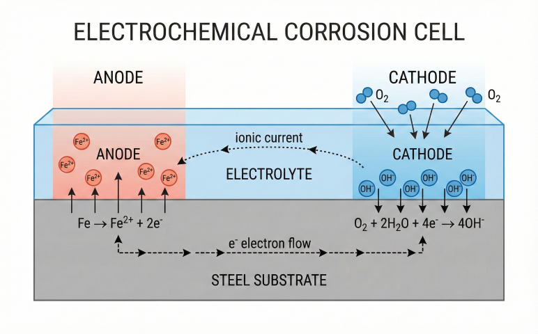
All aqueous corrosion is electrochemical, requiring anodic metal dissolution and cathodic reduction reactions occurring simultaneously at different surface sites.
Electrochemical corrosion cell: anodic dissolution, cathodic reduction, and electron flow through metal.
Fundamental Electrochemistry
Electrochemical Reactions:
Anodic (oxidation): Fe → Fe²⁺ + 2e⁻
Cathodic (reduction):
Aerated neutral: O₂ + 2H₂O + 4e⁻ → 4OH⁻
Acidic/deaerated: 2H⁺ + 2e⁻ → H₂
Overall (aerated): 2Fe + O₂ + 2H₂O → 2Fe(OH)₂ → rust
Corrosion rate from current density:
CR (mpy) = 0.1288 × EW × i_corr / ρ
Where:
i_corr = corrosion current density (μA/cm²)
EW = equivalent weight (g/equivalent)
ρ = metal density (g/cm³)
Sweet Corrosion (CO₂)
Carbon dioxide dissolves in water forming carbonic acid, the primary corrosion mechanism in gas production and gathering systems.
CO₂ Corrosion Chemistry:
CO₂ + H₂O ⇌ H₂CO₃ (carbonic acid, pKa ≈ 6.4)
H₂CO₃ ⇌ H⁺ + HCO₃⁻
Anodic: Fe → Fe²⁺ + 2e⁻
Cathodic: 2H₂CO₃ + 2e⁻ → H₂ + 2HCO₃⁻
Scale: Fe²⁺ + CO₃²⁻ → FeCO₃ (protective above ~60°C)
De Waard-Milliams Correlation (simplified):
log₁₀(CR) = 5.8 − 1710/T + 0.67×log₁₀(pCO₂)
Where: CR in mm/year, T in Kelvin, pCO₂ in bar
Typical uninhibited rates:
pCO₂ = 0.5 bar, 60°C: 2–8 mm/year (80–300 mpy)
Sour Corrosion (H₂S)
Hydrogen sulfide causes both corrosion and cracking. The cracking mechanisms (SSC, HIC, SOHIC) are often more critical than metal loss.
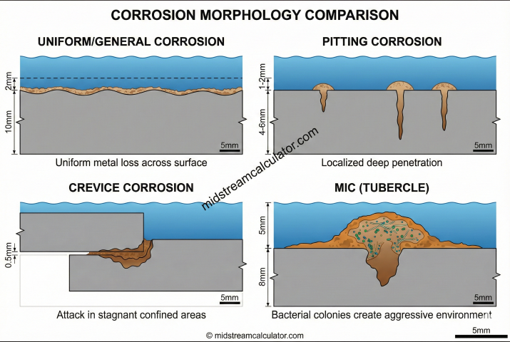
Bacterial activity creates localized aggressive environments. MIC causes severe pitting, often 10–100× general corrosion rates.
SRB (Sulfate-reducing bacteria): Convert SO₄²⁻ to H₂S under biofilms
APB (Acid-producing bacteria): Generate organic acids, drop local pH to 2–3
IOB (Iron-oxidizing bacteria): Form tubercles, create differential aeration cells
Cross-sections comparing uniform corrosion, pitting, crevice corrosion, and MIC tubercle formation.
Corrosion Rate Comparison
Mechanism
Typical Rate
Key Factor
Primary Mitigation
Sweet (CO₂)
10–200 mpy
pCO₂, temperature
Film-forming inhibitors
Sour (H₂S)
5–50 mpy + cracking
pH₂S, pH, hardness
Material selection (MR0175)
Oxygen
50–500 mpy
Dissolved O₂, velocity
Deaeration, scavengers
MIC
10–100 mpy (pitting)
Bacterial population
Biocides, pigging
3. Rate Calculations
Weight Loss Method (ASTM G1-03)
The weight loss method using corrosion coupons remains the industry standard for field corrosion monitoring. Results represent time-averaged corrosion over the exposure period.
ASTM G1 Corrosion Rate Formula:
CR = (K × W) / (A × T × D)
Where:
CR = Corrosion rate
K = Constant (depends on units desired)
W = Weight loss (grams)
A = Exposed surface area (cm²)
T = Exposure time (hours)
D = Material density (g/cm³)
Constants for different units:
K = 3.45 × 10⁶ → CR in mpy (mils per year)
K = 8.76 × 10⁴ → CR in mm/year
K = 8.76 × 10⁷ → CR in μm/year
For carbon steel (D = 7.85 g/cm³):
CR (mpy) = 4.39 × 10⁵ × W / (A × T)
Example: Weight Loss Calculation
Given:
Initial weight: W₁ = 48.526 g
Final weight: W₂ = 48.284 g
Surface area: A = 24.2 cm²
Exposure time: T = 90 days = 2,160 hours
Material: Carbon steel (D = 7.85 g/cm³)
Solution:
Weight loss: W = 48.526 − 48.284 = 0.242 g
CR = (3.45 × 10⁶ × 0.242) / (24.2 × 2,160 × 7.85)
CR = 834,900 / 410,335
CR = 2.03 mpy
Result: 2.0 mpy — Low severity, acceptable rate
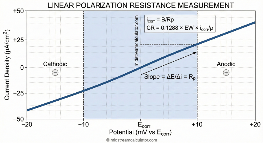
Electrochemical Method (ASTM G102-89)
Linear Polarization Resistance (LPR) and Tafel extrapolation provide instantaneous corrosion rate data, enabling real-time monitoring and rapid inhibitor optimization.
ASTM G102 Corrosion Rate Formula:
CR (mpy) = 0.1288 × EW × i_corr / ρ
Where:
EW = Equivalent weight (g/equivalent)
i_corr = Corrosion current density (μA/cm²)
ρ = Density (g/cm³)
From LPR measurement:
i_corr = B / Rp
Where:
Rp = Polarization resistance (ohm·cm²)
B = Stern-Geary coefficient (mV)
B = (βa × βc) / [2.303 × (βa + βc)]
Typical B for steel in CO₂: 13–26 mV
Example:
Rp = 1,000 ohm·cm², B = 26 mV
i_corr = 26 / 1,000 = 0.026 mA/cm² = 26 μA/cm²
For carbon steel (EW = 27.92, ρ = 7.85):
CR = 0.1288 × 27.92 × 26 / 7.85 = 11.9 mpy
Linear Polarization Resistance (LPR) curve: current vs. potential near E_corr with Rp slope.
Thickness Measurement Method (API 570)
Corrosion Rate from UT Inspection:
CR (mpy) = (t_original − t_measured) × 1000 / years
Example:
Original wall: 0.375 in = 375 mils
Measured wall: 0.358 in = 358 mils
Service time: 12 years
CR = (375 − 358) / 12 = 1.42 mpy
Remaining Life:
Min required thickness: t_min = 0.300 in (for MAWP)
Remaining allowance: 358 − 300 = 58 mils
Remaining life: 58 / 1.42 = 40.8 years
Severity Classification
Rate (mpy)
Classification
Recommended Action
< 1
Negligible
Continue routine monitoring
1–5
Low
Standard inspection intervals
5–10
Moderate
Increase monitoring, review inhibitor
10–20
High
Optimize inhibitor, shorten inspection interval
20–50
Severe
Immediate action: aggressive inhibition or upgrade
> 50
Critical
Consider shutdown, replacement required
Pitting Factor
Pitting Factor Calculation:
PF = Maximum pit depth / Average metal loss
Interpretation:
PF < 2: Predominantly uniform corrosion
PF 2–5: Moderate localized attack
PF > 5: Severe pitting — reduce inspection interval
API 570 Adjustment:
When PF > 2, use pitting rate (not general rate) for
remaining life calculations at pitting locations.
API 570 Inspection Interval
Inspection Interval Calculation:
Interval = (t_current − t_minimum) / (2 × CR)
Or equivalently:
Interval = Remaining Life / 2
API 570 Limits:
• Maximum interval: 10 years
• Minimum interval: Based on risk (typically 5 years for critical)
• Safety factor of 2 built into formula
Example:
t_current = 0.365 in (365 mils)
t_minimum = 0.300 in (300 mils)
CR = 3.5 mpy
Interval = (365 − 300) / (2 × 3.5) = 65 / 7 = 9.3 years
→ Use 9 years or 10-year maximum
4. Standards & Testing
Key Industry Standards
Standard
Title
Application
ASTM G1-03
Preparing, Cleaning, Evaluating Corrosion Test Specimens
Weight loss coupon procedure
ASTM G102-89
Calculation of Corrosion Rates from Electrochemical Measurements
LPR, Tafel, EIS rate calculations
NACE SP0775
Preparation, Installation, Analysis of Corrosion Coupons
Field coupon program design
NACE MR0175
Materials for H₂S Environments (= ISO 15156)
Sour service material selection
API 570
Piping Inspection Code
Inspection intervals, remaining life
API 580/581
Risk-Based Inspection
Inspection prioritization
NACE TM0177
SSC Testing Methods
Sulfide stress cracking evaluation
NACE TM0284
HIC Testing
Hydrogen-induced cracking evaluation
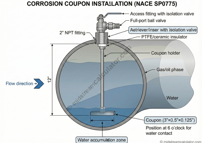
Corrosion Coupon Program (NACE SP0775)
Coupon Specifications:
• Material: Match pipeline metallurgy exactly
• Size: Typically 3" × 0.5" × 0.125" (~24 cm² area)
• Surface: 120-grit finish (reproducible starting point)
• Exposure: 30–90 days typical (longer for low rates)
Installation Requirements:
• Minimum 3 coupons per location (statistical validity)
• Position at pipe bottom (water accumulation)
• Downstream of chemical injection points
• Access fittings per NACE SP0775 specifications
Acceptance Criteria:
< 5 mpy: Acceptable for carbon steel
5–10 mpy: Marginal — increase monitoring
> 10 mpy: Unacceptable — increase inhibitor dosage
Corrosion coupon installation: holder at 6 o'clock position with access fitting per NACE SP0775.
Monitoring Methods Comparison
Method
Response Time
Measures
Limitations
Weight loss coupons
30–90 days
Average rate, pitting
No real-time data
ER probes
Hours to days
Metal loss (cumulative)
No instantaneous rate
LPR probes
Minutes
Instantaneous rate
General corrosion only
UT thickness
Periodic surveys
Actual wall loss
Point measurements
ILI (smart pig)
5–7 year intervals
Full pipe mapping
High cost, piggable lines only
5. Mitigation Strategies
Corrosion Inhibitors
Film-forming inhibitors are the primary internal corrosion control method for carbon steel pipelines. Selection depends on fluid composition and operating conditions.
Economic Decision: Compare life-cycle costs: (1) carbon steel + inhibitor program + increased inspection vs. (2) CRA capital cost + reduced operating costs. Breakeven typically 15–30 years depending on corrosivity and inhibitor costs.
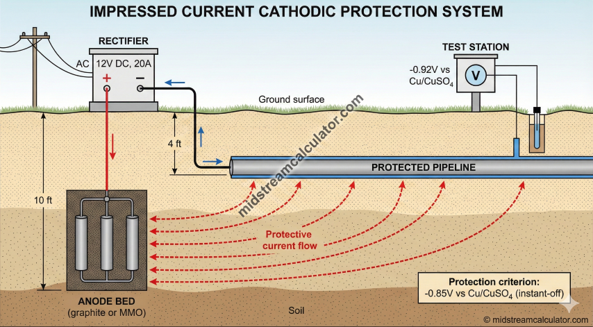
Cathodic Protection (External)
NACE SP0169 Protection Criteria:
1. −850 mV vs Cu/CuSO₄ (instant-off potential)
2. 100 mV polarization from native potential
3. −850 mV with IR drop (where native > −800 mV)
Current Requirement:
I (mA) = A_bare × i_density
Typical current densities (μA/ft²):
• Well-coated pipe: 50–200
• Degraded coating: 500–2,000
• Bare pipe: 5,000–20,000
Cathodic protection system: rectifier, anode bed, current flow, and test station with reference cell.
What methods are used to calculate corrosion rates?+
Corrosion rates are calculated using ASTM G1 weight loss method and ASTM G102 electrochemical methods, both widely used in pipeline integrity programs.
How are corrosion rates used in pipeline inspection planning?+
Corrosion rates determine inspection intervals per API 570, helping engineers schedule maintenance before wall thickness falls below minimum requirements.
What standards govern corrosion rate measurement?+
Key standards include ASTM G1 for weight loss testing, ASTM G102 for electrochemical methods, and NACE standards for field corrosion monitoring.