Evaluate pipeline and midstream project economics using NPV, IRR, and discounted cash flow analysis with WACC-based discount rates for capital investment decisions.
Net Present Value (NPV) analysis is the fundamental method for evaluating capital investments in pipeline and midstream projects. NPV quantifies project value by discounting future cash flows to present value using the company's cost of capital.
Time value of money
Present value concept
Dollar today worth more than dollar tomorrow due to earning potential and risk.
Investment decision
Accept if NPV > 0
Positive NPV means project returns exceed required return; creates value.
Ranking projects
Higher NPV preferred
Among mutually exclusive projects, select highest NPV option.
Capital budgeting
Portfolio optimization
Allocate limited capital to projects with highest NPV per dollar invested.
Key Financial Metrics
NPV (Net Present Value): Sum of discounted cash flows minus initial investment; measures absolute dollar value creation
IRR (Internal Rate of Return): Discount rate that makes NPV = 0; measures percentage return
PI (Profitability Index): NPV / Initial Investment; measures value per dollar invested
Payback Period: Years to recover initial investment (see payback-analysis-fundamentals.html)
WACC (Weighted Average Cost of Capital): Company's blended cost of debt and equity financing
Why NPV is preferred: NPV directly measures dollar value created, accounts for all cash flows, incorporates time value of money, and uses realistic discount rate (WACC). Superior to payback period or accounting rate of return for capital budgeting decisions.
NPV Decision Framework
NPV Result
Meaning
Decision
NPV > 0
Project returns exceed cost of capital
Accept - creates shareholder value
NPV = 0
Project returns equal cost of capital
Indifferent - no value creation/destruction
NPV < 0
Project returns below cost of capital
Reject - destroys shareholder value
NPV₁ > NPV₂
Mutually exclusive projects
Select Project 1 (higher NPV)
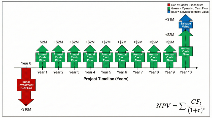
Types of Cash Flows
Project cash flow timeline illustrating initial investment, annual operating cash flows, and terminal salvage value used in NPV calculations.
Terminal cash flow (Year N): Salvage value, working capital recovery, decommissioning costs
Tax effects: Depreciation tax shield, capital gains/losses on disposal
Common Pipeline Investment Types
Project Type
Typical Investment
Cash Flow Profile
Project Life
Greenfield transmission pipeline
$500M - $5B
Large upfront CAPEX, stable long-term revenue
30-50 years
Lateral extension
$10M - $100M
Moderate CAPEX, incremental revenue
20-30 years
Compressor station upgrade
$20M - $200M
CAPEX, reduced fuel costs, increased capacity
15-25 years
Integrity/replacement
$5M - $50M
CAPEX, avoided failure costs, maintained revenue
10-20 years
Metering/automation
$1M - $10M
CAPEX, reduced labor, improved accuracy
10-15 years
2. NPV Calculation
NPV equals the sum of all future cash flows discounted to present value minus the initial investment.
NPV Formula
Net Present Value:
NPV = Σ [CF_t / (1 + r)^t] - Initial Investment
Or expanded:
NPV = -CF₀ + CF₁/(1+r)¹ + CF₂/(1+r)² + ... + CF_N/(1+r)^N
Where:
NPV = Net present value ($)
CF_t = Cash flow in year t ($)
r = Discount rate (WACC, decimal)
t = Time period (years)
N = Project life (years)
CF₀ = Initial investment (negative cash flow)
Alternative form with salvage value:
NPV = -I₀ + Σ(t=1 to N) [CF_t/(1+r)^t] + S_N/(1+r)^N
Where:
I₀ = Initial investment
S_N = Salvage value at end of year N
Discount Factor
Present Value Factor:
PV Factor = 1 / (1 + r)^t
This is the present value of $1 received in year t.
Example discount factors at r = 10%:
Year 1: PV = 1/1.10 = 0.9091 (each dollar worth $0.91 today)
Year 5: PV = 1/(1.10)^5 = 0.6209
Year 10: PV = 1/(1.10)^10 = 0.3855
Year 20: PV = 1/(1.10)^20 = 0.1486
Note: Distant cash flows heavily discounted (Year 20 dollar worth only $0.15 today)
IRR Definition:
Find IRR such that:
NPV = 0 = Σ [CF_t / (1 + IRR)^t] - I₀
For the lateral example above:
0 = -37 + 6/(1+IRR)¹ + 6/(1+IRR)² + ... + 6/(1+IRR)²⁰ + 5/(1+IRR)²⁰
Solve iteratively (trial and error or Excel IRR function):
IRR = 15.1%
Decision rule:
If IRR > WACC (15.1% > 10%), accept project ✓
If IRR < WACC, reject project
Note: IRR = 15.1% means project returns 15.1% annually,
exceeding 10% cost of capital by 5.1 percentage points.
Profitability Index
Profitability Index (PI):
PI = NPV / Initial Investment
Or:
PI = PV(Cash Inflows) / PV(Cash Outflows)
For lateral example:
PI = 14.82 / 37 = 0.40 = 40%
Interpretation: Every $1 invested creates $0.40 of value
Or: PV of inflows is 1.40× initial investment
Decision rule:
PI > 0: Accept (equivalent to NPV > 0)
PI < 0: Reject
Use for capital rationing: Rank projects by PI when budget limited
Unequal Cash Flows
Many projects have varying cash flows over time:
Example: Compressor Station with Increasing Tariffs
Year 0: CAPEX = -$50M
Year 1-5: CF = $8M/year
Year 6-10: CF = $10M/year (tariff increase)
Year 11-15: CF = $12M/year
Year 15: Salvage = $8M
Discount rate: r = 9%
Calculate NPV by summing discounted cash flows:
Years 1-5: PV = 8 × [(1-1.09^-5)/0.09] = 8 × 3.8897 = $31.12M
Years 6-10: PV = 10 × [(1-1.09^-5)/0.09] × (1.09)^-5 = 10 × 3.8897 × 0.6499 = $25.28M
Years 11-15: PV = 12 × [(1-1.09^-5)/0.09] × (1.09)^-10 = 12 × 3.8897 × 0.4224 = $19.72M
Salvage: PV = 8 / (1.09)^15 = 8 × 0.2745 = $2.20M
NPV = -50 + 31.12 + 25.28 + 19.72 + 2.20 = $28.32M ✓
Project highly attractive with NPV = $28M
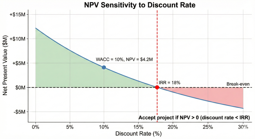
NPV profile showing how net present value decreases as discount rate increases, crossing zero at the internal rate of return (IRR = 18%).
Mid-Year Convention
For more accuracy, assume cash flows occur mid-year instead of year-end:
Mid-Year Discounting:
Standard (year-end): PV = CF / (1+r)^t
Mid-year: PV = CF / (1+r)^(t-0.5)
Effect: Increases NPV slightly (cash received sooner)
For Year 1 cash flow at 10% discount:
Year-end PV: CF / 1.10 = 0.9091 × CF
Mid-year PV: CF / 1.10^0.5 = CF / 1.0488 = 0.9535 × CF
Difference: ~4.8% higher PV with mid-year convention
Use mid-year for monthly/continuous cash flows (tariff revenue)
Use year-end for annual lump sums (tax payments)
Common NPV Pitfalls
Ignoring taxes: Use after-tax cash flows; depreciation creates tax shield
Sunk costs: Exclude past expenditures (e.g., feasibility studies already paid)
Allocated overhead: Include only incremental costs caused by project
Inflation: Match nominal cash flows with nominal discount rate, or real with real
Working capital: Include working capital investment and recovery
Opportunity cost: Include forgone alternatives (e.g., land could be sold)
Tax considerations: Pipelines use MACRS depreciation (15-year or 20-year property). Depreciation is non-cash expense that reduces taxable income, creating tax shield. Tax shield value = Depreciation × Tax Rate. Must include in cash flow analysis.
3. Discount Rate & WACC
The discount rate represents the opportunity cost of capital - the return investors could earn on alternative investments of similar risk. WACC is the most common discount rate for corporate investments.
Weighted Average Cost of Capital (WACC)
WACC Formula:
WACC = (E/V) × r_e + (D/V) × r_d × (1 - T_c)
Where:
WACC = Weighted average cost of capital
E = Market value of equity
D = Market value of debt
V = E + D = Total firm value
r_e = Cost of equity (required return on equity)
r_d = Cost of debt (interest rate on debt)
T_c = Corporate tax rate
(1 - T_c) = Tax shield on debt interest
Interpretation:
- First term: Cost of equity, weighted by equity proportion
- Second term: After-tax cost of debt, weighted by debt proportion
- Debt is tax-deductible, so after-tax cost is r_d × (1-T_c)
Cost of Equity - CAPM
Cost of equity calculated using Capital Asset Pricing Model:
Fisher Equation:
(1 + r_nominal) = (1 + r_real) × (1 + inflation)
Or approximately:
r_nominal ≈ r_real + inflation
Where:
r_nominal = Nominal discount rate (includes inflation)
r_real = Real discount rate (inflation-adjusted)
inflation = Expected inflation rate
Example: If WACC = 9% nominal and inflation = 2.5%
r_real = (1.09 / 1.025) - 1 = 6.34%
Consistency requirement:
- Nominal cash flows → use nominal discount rate
- Real cash flows → use real discount rate
Most corporate analyses use nominal rates and nominal cash flows
WACC limitations: WACC assumes constant capital structure and risk over project life. For projects that change company risk profile or financing, use APV (Adjusted Present Value) method. For very long projects (30+ years), consider declining discount rate (lower rates for distant cash flows).
4. Sensitivity Analysis
Sensitivity analysis examines how NPV changes when key assumptions vary. Essential for understanding project risk and identifying critical success factors.
One-Way Sensitivity
Vary one input at a time while holding others constant:
Example: Pipeline Lateral Sensitivity
Base case:
- Initial investment: $37M
- Annual revenue: $8M
- Annual OPEX: $2M
- Discount rate: 10%
- Project life: 20 years
- Base NPV: $14.82M
Sensitivity to revenue (±20%):
Revenue at $6.4M/yr (-20%): NPV = -$2.26M (REJECT)
Revenue at $8.0M/yr (base): NPV = $14.82M
Revenue at $9.6M/yr (+20%): NPV = $31.90M
Sensitivity to discount rate:
At 8% WACC: NPV = $21.63M
At 10% WACC (base): NPV = $14.82M
At 12% WACC: NPV = $9.17M
At 15% WACC: NPV = $0.40M (barely positive)
Critical insight: Project very sensitive to revenue; less sensitive to WACC
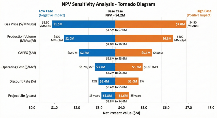
Tornado Diagram
Bar chart showing impact of each variable on NPV:
Tornado diagram ranking input variables by their impact on NPV. Gas price and production volume are the most sensitive variables requiring careful estimation.
Break-Even Revenue:
For lateral example, find revenue that gives NPV = 0:
0 = -37 + (Rev - 2) × [(1 - 1.10^-20) / 0.10] + 0.74
0 = -37 + (Rev - 2) × 8.514 + 0.74
0 = -36.26 + 8.514 × Rev - 17.03
0 = 8.514 × Rev - 53.29
Rev_breakeven = 53.29 / 8.514 = $6.26M/year
Interpretation: Need at least $6.26M annual revenue for positive NPV
Base case $8M is 27% above breakeven (good margin)
Break-even capacity (if tariff = $2/Mcf):
Q_breakeven = 6.26M / $2 = 3.13 MMcf/day
Monte Carlo Simulation
Probabilistic analysis using random sampling:
Monte Carlo NPV Simulation:
Define probability distributions for key variables:
- Revenue: Normal(μ=$8M, σ=$1.5M)
- OPEX: Normal(μ=$2M, σ=$0.4M)
- CAPEX: Triangular(min=$33M, mode=$37M, max=$42M)
- Discount rate: Fixed at 10%
Run 10,000 simulations:
1. Randomly sample revenue, OPEX, CAPEX from distributions
2. Calculate NPV for each draw
3. Compile NPV distribution
Results (example):
- Mean NPV: $14.5M
- Median NPV: $14.8M
- Std Dev: $8.2M
- P(NPV > 0): 92% (8% risk of loss)
- P(NPV > $20M): 25%
- 5th percentile NPV: -$2.1M (worst case)
- 95th percentile NPV: $29.3M (best case)
Decision: 92% probability of positive NPV supports investment
Decision Trees for Sequential Decisions
Analyze projects with decision points over time:
Example: Two-Phase Pipeline Expansion
Year 0: Decide whether to build Phase 1 ($30M)
Year 3: If demand high, build Phase 2 ($40M); if low, abandon
Phase 1 alone:
- High demand (60% prob): NPV = $20M
- Low demand (40% prob): NPV = -$5M
Phase 2 (if built in Year 3 after high demand):
- Additional NPV = $35M (discounted to Year 3)
- PV at Year 0 = 35M / (1.10)^3 = $26.3M
Decision tree:
Year 0: Build Phase 1
Year 3 (if high demand): Build Phase 2
Year 3 (if low demand): Do not build Phase 2
Expected NPV:
E(NPV) = 0.60 × (20 + 26.3) + 0.40 × (-5)
E(NPV) = 0.60 × 46.3 + 0.40 × (-5)
E(NPV) = 27.78 - 2.0 = $25.78M
Option value from flexibility: $25.78M vs. $11M (Phase 1 only expected NPV)
Real options: Projects with flexibility (expand, contract, abandon, delay) have option value beyond simple NPV. Use decision trees or real options analysis (Black-Scholes for deferral option) to capture value of managerial flexibility in uncertain environments.
5. Practical Applications
Capital Budgeting - Portfolio Selection
Allocate limited capital across competing projects:
Example: $100M Capital Budget, 5 Projects Available
Project A: Lateral extension
- CAPEX: $37M, NPV: $14.8M, IRR: 15.1%, PI: 0.40
Project B: Compressor upgrade
- CAPEX: $25M, NPV: $8.2M, IRR: 14.5%, PI: 0.33
Project C: Integrity replacement
- CAPEX: $15M, NPV: $3.5M, IRR: 11.8%, PI: 0.23
Project D: Metering system
- CAPEX: $8M, NPV: $4.1M, IRR: 18.2%, PI: 0.51
Project E: Greenfield pipeline
- CAPEX: $65M, NPV: $22.0M, IRR: 13.2%, PI: 0.34
Ranking by NPV:
1. Project E: $22.0M
2. Project A: $14.8M
3. Project B: $8.2M
4. Project D: $4.1M
5. Project C: $3.5M
Total NPV if all accepted: $52.6M
Total CAPEX required: $150M (exceeds $100M budget)
Solution 1: Rank by NPV (accept E, A, B, D)
Total CAPEX: $135M (still exceeds budget)
Solution 2: Rank by PI (value per dollar invested)
1. Project D: PI = 0.51
2. Project A: PI = 0.40
3. Project E: PI = 0.34
4. Project B: PI = 0.33
5. Project C: PI = 0.23
Accept D + A + B: CAPEX = $70M, Total NPV = $27.1M ✓
Add C: CAPEX = $85M, Total NPV = $30.6M ✓
Optimal portfolio: D, A, B, C for $85M CAPEX, $30.6M NPV
Remaining $15M for smaller projects or reserve
Best practices: Always perform sensitivity analysis on key assumptions (tariff, throughput, CAPEX). Use probability-weighted scenarios for high-uncertainty projects. Include real options value for flexible projects (phased expansion, abandonment options). Conservative assumptions better than optimistic for capital approval.
Industry Standards and References
FERC regulations: Federal Energy Regulatory Commission tariff and rate-making guidelines for interstate pipelines
IRS Publication 946: MACRS depreciation for pipeline assets (15-year or 20-year property)
SEC guidance: Proved reserves and project valuation disclosure requirements
GAAP/IFRS: Accounting standards for capital investments and impairment testing
Project Management Institute (PMI): Economic analysis standards and best practices