Calculate simple and discounted payback periods, evaluate investment criteria using NPV and IRR, and understand time value of money for pipeline and midstream project justification.
Payback period is the time required for cumulative cash inflows from a project to equal the initial investment. It is one of the most widely used screening tools in capital budgeting for pipeline and midstream projects.
Pipeline expansions
Capacity additions
New compressor stations, looping, diameter increases justified by throughput revenue.
Efficiency projects
Energy savings
VFDs, insulation upgrades, heat recovery systems with utility cost reduction.
Reliability improvements
Maintenance reduction
Equipment upgrades that reduce downtime and maintenance costs.
Safety & compliance
Risk mitigation
Integrity management, leak detection, safety systems justified by avoided costs.
Key Concepts
Initial investment (I₀): Total capital expenditure including equipment, installation, engineering, and startup costs
Cash flow (CF): Net annual cash inflow from project (revenue increase or cost savings minus operating costs)
Time value of money: Principle that a dollar today is worth more than a dollar in the future due to earning potential
Discount rate (r): Required rate of return reflecting risk and cost of capital
Why payback analysis matters: Simple payback provides quick go/no-go screening. Discounted payback accounts for time value of money. Combined with NPV and IRR, these metrics form a comprehensive investment decision framework.
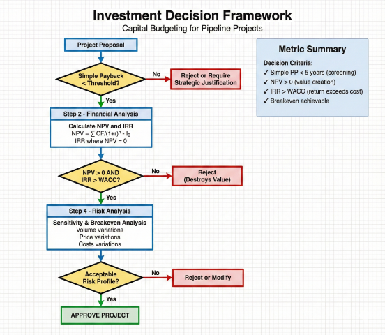
Investment decision framework integrating payback period screening with NPV, IRR, and risk analysis for capital project evaluation
Advantages of Payback Method
Simplicity: Easy to calculate and explain to non-financial stakeholders
Risk indicator: Shorter payback means faster capital recovery and lower risk
Liquidity focus: Emphasizes cash recovery important for capital-constrained companies
Screening tool: Quick filter for obviously poor projects before detailed analysis
Limitations of Payback Method
Ignores cash flows beyond payback: Doesn't consider project life or total profitability
No time value (simple): Simple payback doesn't discount future cash flows
Arbitrary cutoff: Payback threshold (e.g., 3 years) may not align with value creation
Biased against long-term projects: May reject valuable long-lived infrastructure
2. Simple Payback Period
Simple payback period is the most basic capital budgeting metric. It calculates the time to recover initial investment assuming equal annual cash flows, without considering time value of money.
When cash flows vary by year, calculate cumulative cash flow and find when it equals initial investment:
Cumulative Cash Flow Method:
Cumulative CF_n = Σ(CF₁ + CF₂ + ... + CF_n)
Find n where Cumulative CF_n ≥ I₀
If recovery occurs partway through year n:
PP = (n-1) + (I₀ - Cumulative CF_(n-1)) / CF_n
Example with varying cash flows:
Initial investment: $800,000
Year 1: $150,000 → Cumulative: $150,000
Year 2: $200,000 → Cumulative: $350,000
Year 3: $250,000 → Cumulative: $600,000
Year 4: $300,000 → Cumulative: $900,000
Recovery occurs in Year 4:
Remaining after Year 3: $800,000 - $600,000 = $200,000
Fraction of Year 4: $200,000 / $300,000 = 0.67
Payback Period = 3 + 0.67 = 3.67 years
Typical Payback Thresholds by Industry
Project Type
Typical Threshold
Rationale
Energy efficiency (motors, VFDs)
2-3 years
Technology obsolescence, short economic life
Process improvements
3-5 years
Moderate risk, proven technology
Pipeline capacity expansion
4-7 years
Long-term contracts, regulated returns
New facilities (greenfield)
5-10 years
30+ year design life, strategic infrastructure
Safety/environmental compliance
Not applicable
Mandatory; justify via risk reduction, not payback
R&D / pilot projects
N/A or 1-2 years
High uncertainty; very short payback or strategic value
Pipeline Expansion Example
A pipeline operator considers adding a compressor station to increase throughput from 500 MMcf/d to 650 MMcf/d.
Project Data:
Compressor station cost: $12,000,000
Additional throughput: 150 MMcf/d
Transportation tariff: $0.50/Mcf
Operating days: 350 days/year
Annual O&M cost: $1,200,000/year
Annual Revenue Increase:
Volume = 150,000 Mcf/day × 350 days = 52,500,000 Mcf/year
Revenue = 52,500,000 × $0.50 = $26,250,000/year
Net Annual Cash Flow:
CF = $26,250,000 - $1,200,000 = $25,050,000/year
Simple Payback:
PP = $12,000,000 / $25,050,000 = 0.48 years = 5.8 months
Interpretation: Very attractive project with sub-1-year payback, assuming capacity can be sold.
Energy Efficiency Example
Replace existing fixed-speed compressor motor with VFD to reduce power consumption:
Project Data:
VFD installed cost: $85,000
Current power consumption: 400 kW average
Expected reduction: 15%
Power cost: $0.10/kWh
Operating hours: 8,000 hr/year
Annual Energy Savings:
kWh saved = 400 kW × 0.15 × 8,000 hr = 480,000 kWh/year
Cost savings = 480,000 × $0.10 = $48,000/year
Simple Payback:
PP = $85,000 / $48,000 = 1.77 years
Interpretation: Acceptable payback for energy efficiency. Project likely approved.
Rule of thumb: For midstream operators, simple payback < 3 years is considered excellent, 3-5 years is good, 5-7 years is marginal. Projects > 7 years require strategic justification beyond financial return.
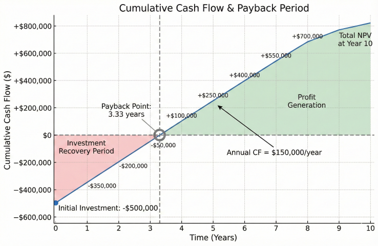
Cumulative cash flow curve illustrating payback period where cumulative returns equal initial investment
3. Discounted Payback Period
Discounted payback period accounts for the time value of money by discounting future cash flows to present value. This provides a more conservative and financially rigorous assessment than simple payback.
Present Value of Cash Flows
Present Value Formula:
PV = CF / (1 + r)ⁿ
Where:
PV = Present value of cash flow ($)
CF = Future cash flow in year n ($)
r = Discount rate (decimal)
n = Year number
Cumulative Present Value:
Cumulative PV_n = Σ [CF_i / (1 + r)ⁱ] for i = 1 to n
Find n where Cumulative PV_n ≥ I₀
Discounted Payback Calculation
Step-by-Step Process:
1. Select appropriate discount rate (WACC or hurdle rate)
2. Calculate present value of each year's cash flow
3. Sum present values cumulatively by year
4. Find year when cumulative PV equals initial investment
5. Interpolate if recovery occurs mid-year
Interpolation Formula:
DPP = (n-1) + [(I₀ - Cumulative PV_(n-1)) / PV_n]
Where DPP = Discounted payback period (years)
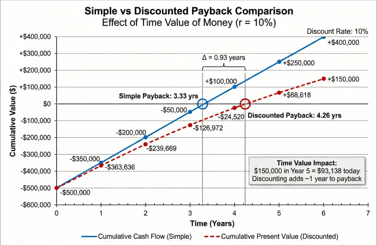
Comparison Example: Simple vs. Discounted Payback
Project with $500,000 initial investment, 10% discount rate:
Year
Cash Flow
Cumulative CF (Simple)
PV Factor (1+0.10)ⁿ
Present Value
Cumulative PV (Discounted)
0
-$500,000
-$500,000
1.000
-$500,000
-$500,000
1
$150,000
-$350,000
1.100
$136,364
-$363,636
2
$150,000
-$200,000
1.210
$123,967
-$239,669
3
$150,000
-$50,000
1.331
$112,697
-$126,972
4
$150,000
$100,000
1.464
$102,452
-$24,520
5
$150,000
$250,000
1.611
$93,138
$68,618
Simple Payback Calculation:
Recovery in Year 4: 3 + ($50,000 / $150,000) = 3.33 years
Discounted Payback Calculation:
Recovery in Year 5: 4 + ($24,520 / $93,138) = 4.26 years
Difference: 4.26 - 3.33 = 0.93 years longer
Interpretation: Discounting increases payback by ~1 year due to time value of money.
The $150,000 received in Year 5 is worth only $93,138 today.
Selecting the Discount Rate
The discount rate should reflect the project's risk and opportunity cost of capital:
Discount Rate Type
Typical Range
When to Use
WACC (Weighted Average Cost of Capital)
8-12%
Standard projects with average risk profile
Hurdle rate (WACC + risk premium)
12-18%
High-risk projects, new technologies, uncertain markets
Weighted Average Cost of Capital:
WACC = (E/V) × Re + (D/V) × Rd × (1 - Tc)
Where:
E = Market value of equity
D = Market value of debt
V = E + D (total value)
Re = Cost of equity
Rd = Cost of debt
Tc = Corporate tax rate
Example Calculation:
Equity: $100M at 12% cost
Debt: $40M at 6% cost
Tax rate: 25%
E/V = $100M / $140M = 71.4%
D/V = $40M / $140M = 28.6%
WACC = 0.714 × 12% + 0.286 × 6% × (1 - 0.25)
WACC = 8.57% + 1.29% = 9.86% ≈ 10%
Impact of discount rate: Higher discount rates penalize distant cash flows more heavily, increasing discounted payback period. A 5% increase in discount rate typically adds 0.5-1.5 years to payback for 5-10 year projects.
Simple vs discounted payback comparison showing how time value of money extends payback period by approximately one year at 10% discount rate
When Projects Never Pay Back
Some projects have negative NPV and never achieve discounted payback:
Example of No Payback:
Initial investment: $1,000,000
Annual cash flow: $80,000/year for 20 years
Discount rate: 12%
PV of cash flows = $80,000 × [PV annuity factor, 12%, 20 years]
PV = $80,000 × 7.469 = $597,520
Since $597,520 < $1,000,000, project never pays back in PV terms.
NPV = -$1,000,000 + $597,520 = -$402,480 (reject project)
4. Breakeven Analysis
Breakeven analysis determines the minimum performance level (throughput, price, cost savings) required for a project to achieve target payback period or NPV = 0.
Breakeven Throughput
For capacity expansion projects, calculate minimum volume needed to recover investment:
Breakeven Volume Calculation:
Total Annual Cost = (I₀ / PP) + Annual O&M
Required Volume = Total Annual Cost / Unit Margin
Where:
I₀ = Initial investment
PP = Target payback period (years)
Unit Margin = Tariff revenue per unit - variable cost per unit
Example - Pipeline Looping:
Investment: $25,000,000
Target payback: 5 years
Annual O&M: $800,000/year
Tariff: $0.75/Mcf
Variable cost: $0.05/Mcf
Annual cost to recover = $25,000,000 / 5 + $800,000 = $5,800,000
Unit margin = $0.75 - $0.05 = $0.70/Mcf
Breakeven volume = $5,800,000 / $0.70 = 8,285,714 Mcf/year
= 22,710 Mcf/day (assuming 365 days)
If project adds 200 MMcf/d capacity and can sell 25 MMcf/d or more,
project exceeds breakeven requirement.
Breakeven Tariff/Price
Determine minimum price or tariff needed for acceptable economics:
Evaluate how payback period changes with key variables:
Scenario
Volume (MMcf/d)
Tariff ($/Mcf)
O&M ($/yr)
Annual CF
Payback (yrs)
Base Case
50
$0.80
$2.0M
$12.6M
3.97
Low volume (-20%)
40
$0.80
$2.0M
$9.68M
5.17
Low tariff (-15%)
50
$0.68
$2.0M
$10.41M
4.80
High O&M (+30%)
50
$0.80
$2.6M
$12.0M
4.17
Optimistic (all favorable)
60
$0.90
$1.8M
$17.13M
2.92
Pessimistic (all unfavorable)
40
$0.68
$2.6M
$7.33M
6.83
Assumes $50M investment, 365 operating days/year
Monte Carlo Simulation for Risk Assessment
For high-value projects, use probabilistic analysis to quantify payback period uncertainty:
Monte Carlo Approach:
1. Define probability distributions for uncertain variables:
- Volume: Normal distribution, mean 50 MMcf/d, std dev 8 MMcf/d
- Tariff: Triangular distribution, min $0.65, most likely $0.80, max $0.95
- O&M: Log-normal distribution, mean $2.0M, std dev $0.4M
2. Run 10,000 simulations, randomly sampling from distributions
3. Calculate payback period for each simulation
4. Analyze results:
- P10 (10th percentile): 3.1 years (optimistic)
- P50 (median): 4.2 years (expected)
- P90 (90th percentile): 6.8 years (pessimistic)
- Probability of payback < 5 years: 72%
5. Decision: Accept if P90 < management threshold (e.g., 7 years)
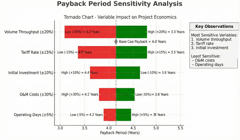
Sensitivity tornado chart identifying volume throughput and tariff rate as the most critical variables affecting payback period
5. Investment Decision Criteria
Payback period should be used alongside other financial metrics for comprehensive project evaluation. The primary criteria are Net Present Value (NPV) and Internal Rate of Return (IRR).
Communicate returns to management; compare to hurdle rates
Profitability Index
Measures value per dollar invested; good for capital rationing
Doesn't show absolute value; can conflict with NPV
Budget constraints; ranking projects with different scales
Profitability Index (PI)
Profitability Index Formula:
PI = PV of Future Cash Flows / Initial Investment
PI = [Σ (CF_t / (1+r)ᵗ)] / I₀
Decision Rule:
PI > 1.0 → Accept (NPV > 0)
PI < 1.0 → Reject (NPV < 0)
PI = 1.0 → Indifferent (NPV = 0)
Example:
PV of cash flows: $1,200,000
Investment: $1,000,000
PI = $1,200,000 / $1,000,000 = 1.20
Interpretation: Project returns $1.20 for every $1.00 invested (20% value creation)
Integrated Decision Framework
Comprehensive project evaluation using multiple criteria:
Project
Investment
Simple PP
Disc. PP
NPV @10%
IRR
PI
Decision
Compressor station
$8M
3.2 yr
4.1 yr
$3.5M
18.2%
1.44
Accept - All metrics favorable
VFD retrofit
$250K
2.8 yr
3.4 yr
$75K
24.5%
1.30
Accept - Excellent returns
Pipeline looping
$40M
6.5 yr
8.9 yr
$2.1M
11.8%
1.05
Marginal - Low but positive NPV
Meter upgrades
$1.2M
8.1 yr
Never
-$350K
7.2%
0.71
Reject - NPV < 0, IRR < WACC
SCADA system
$3M
N/A
N/A
-$1.2M
N/A
N/A
Accept - Safety/reliability, not financial
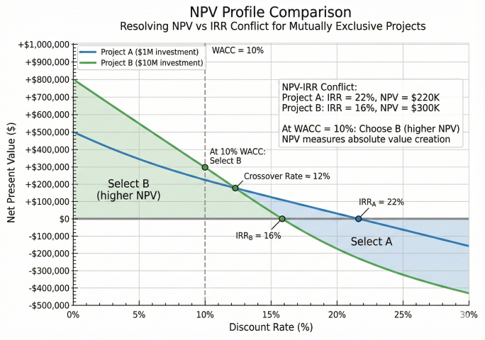
Decision Conflicts: NPV vs. IRR
For mutually exclusive projects of different scales, NPV and IRR can give conflicting rankings:
Example of NPV-IRR Conflict:
Project A (Small):
Investment: $1,000,000
NPV: $400,000
IRR: 22%
Project B (Large):
Investment: $10,000,000
NPV: $2,500,000
IRR: 16%
Analysis:
- By IRR: Select Project A (22% > 16%)
- By NPV: Select Project B ($2.5M > $0.4M)
Correct Decision: Select Project B
NPV measures absolute value creation. Project B adds $2.5M vs. $0.4M.
Even though A has higher percentage return, B creates more shareholder value.
When to use IRR: Comparing projects of similar scale and timing.
When to use NPV: Mutually exclusive projects of different scales (use NPV).
NPV profile crossover chart demonstrating how NPV and IRR can give conflicting rankings for mutually exclusive projects of different scales
Decision Tree for Project Approval
Recommended Decision Process:
Step 1: Calculate Simple Payback
- If PP > 10 years → Likely reject (unless strategic)
- If PP ≤ 3 years → Proceed to Step 2 (strong candidate)
- If 3 < PP ≤ 10 → Proceed to Step 2 (requires detailed analysis)
Step 2: Calculate NPV and IRR
- If NPV > 0 AND IRR > WACC → Accept
- If NPV < 0 OR IRR < WACC → Reject
- If NPV ≈ 0 → Sensitivity analysis required
Step 3: Sensitivity and Risk Analysis
- Identify key uncertainties (volume, price, costs)
- Calculate breakeven values
- Assess probability of achieving targets
- Consider strategic value, competitive position, regulatory factors
Step 4: Management Review
- Present all metrics with sensitivity cases
- Recommend accept/reject with rationale
- Identify key assumptions and risks
- Propose monitoring metrics for post-approval tracking
Best practice: Use simple payback for initial screening, NPV as primary decision criterion, IRR for communication to management, and discounted payback for risk assessment. No single metric tells the complete story.