Gas Transmission

Pipeline Hydraulics

Predict gas flow, pressure profiles, and compressor needs with the right equation for your line size and operating window.

Launch calculator Design checks

Equation fit

Weymouth / Panhandle

Pick based on diameter and Re range for best accuracy.

Gas behavior

Compressible

Use Z-corrected forms and average pressure assumptions.

Profile

Nonlinear drop

dP/dL steepest at inlet as velocity is highest.

1. Flow Fundamentals
2. Gas Flow Equations
3. Friction Factors
4. Elevation Effects
5. Design Considerations

Use this when you need to:

Screen throughput vs. pressure for a new gas line.
Select the right equation for size/pressure regime.
Estimate compressor suction/ discharge bounds.

1. Flow Fundamentals

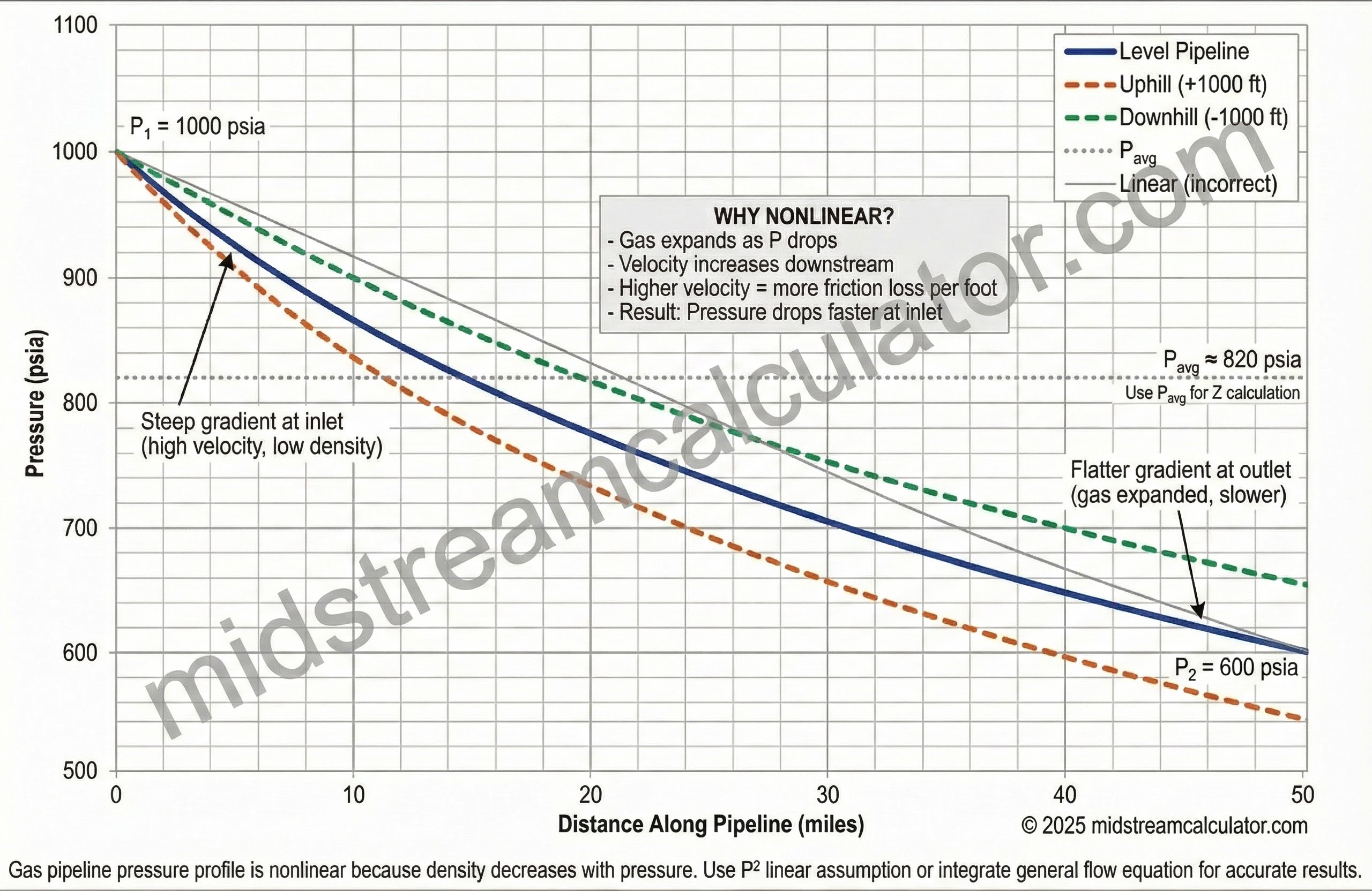
Gas pipeline hydraulics relates pressure drop to flow rate, pipe geometry, and gas properties. Unlike incompressible liquids, gas density varies with pressure, requiring specialized equations.

Key Parameters

Pressure

P₁ / P₂

Inlet/outlet pressures (psia) drive flow and Z.

Geometry

D, L

Inside diameter and line length; check internal roughness.

Gas properties

SG, Z, T

Specific gravity, compressibility, flowing temperature.

Flow regime

Re

Almost always turbulent; Re sets friction factor.

Pipeline pressure profile showing non-linear drop from P₁ to P₂ with average pressure and elevation-adjusted cases.

Reynolds Number

Re = 0.7 × (Q × SG) / (D × μ) Where: Re = Reynolds number (dimensionless) Q = Flow rate (SCFD) SG = Specific gravity D = Inside diameter (inches) μ = Viscosity (cp) Turbulent flow: Re > 4,000 (typical for pipelines)

Operating regime

Re ≫ 4,000

Transmission lines are almost always fully turbulent.

Z handling

Use P_avg

Estimate compressibility at average pressure and flowing T.

Pressure ratio

P₂/P₁

Stay within equation’s tested ratios; flag aggressive drops.

2. Gas Flow Equations

Several empirical equations relate flow rate to pressure drop. Each has specific applications and accuracy ranges.

General Flow Equation

Q = 77.54 × (T_b/P_b) × [(P₁² - P₂²) / (SG × T × L × Z)]^0.5 × D^2.5 / f^0.5 Where: Q = Flow rate (SCFD) T_b = Base temperature (520°R standard) P_b = Base pressure (14.73 psia standard) f = Friction factor (Moody)

Weymouth Equation

Q = 433.5 × E × (T_b/P_b) × [(P₁² - P₂²) / (SG × T × L × Z)]^0.5 × D^2.667 Where: E = Pipeline efficiency (0.85–0.95 typical) Best for: High-pressure, large-diameter transmission lines Diameter range: > 6 inches

Select

Choose equation. Weymouth for large, high-P; Panhandle A/B for moderate to high Re; AGA for detailed compressibility.

Normalize

Use base conditions. Keep T_b and P_b consistent (usually 520°R and 14.73 psia).

Check range

Stay in-bounds. Validate D/Re ranges and pressure ratios; flag extrapolation.

Panhandle A Equation

Q = 435.87 × E × (T_b/P_b)^1.0788 × [(P₁² - P₂²) / (SG^0.8539 × T × L × Z)]^0.5394 × D^2.6182 Best for: Medium to large diameter, moderate Reynolds numbers Re range: 5×10⁶ to 11×10⁶

Panhandle B Equation

Q = 737 × E × (T_b/P_b)^1.02 × [(P₁² - P₂²) / (SG^0.961 × T × L × Z)]^0.51 × D^2.53 Best for: Large diameter, high Reynolds numbers Re range: > 4×10⁶

Equation Comparison

Equation	Diameter	Pressure	Flow Type
Weymouth	> 6"	High (> 100 psig)	Fully turbulent
Panhandle A	4"–24"	Moderate–High	Partially turbulent
Panhandle B	> 12"	High	Fully turbulent
AGA (General)	Any	Any	Most accurate

Which equation? Weymouth is conservative (predicts lower capacity). Panhandle B is optimistic. AGA with Colebrook friction factor is most accurate but requires iteration. For quick estimates, Panhandle A is a good middle ground.

3. Friction Factors

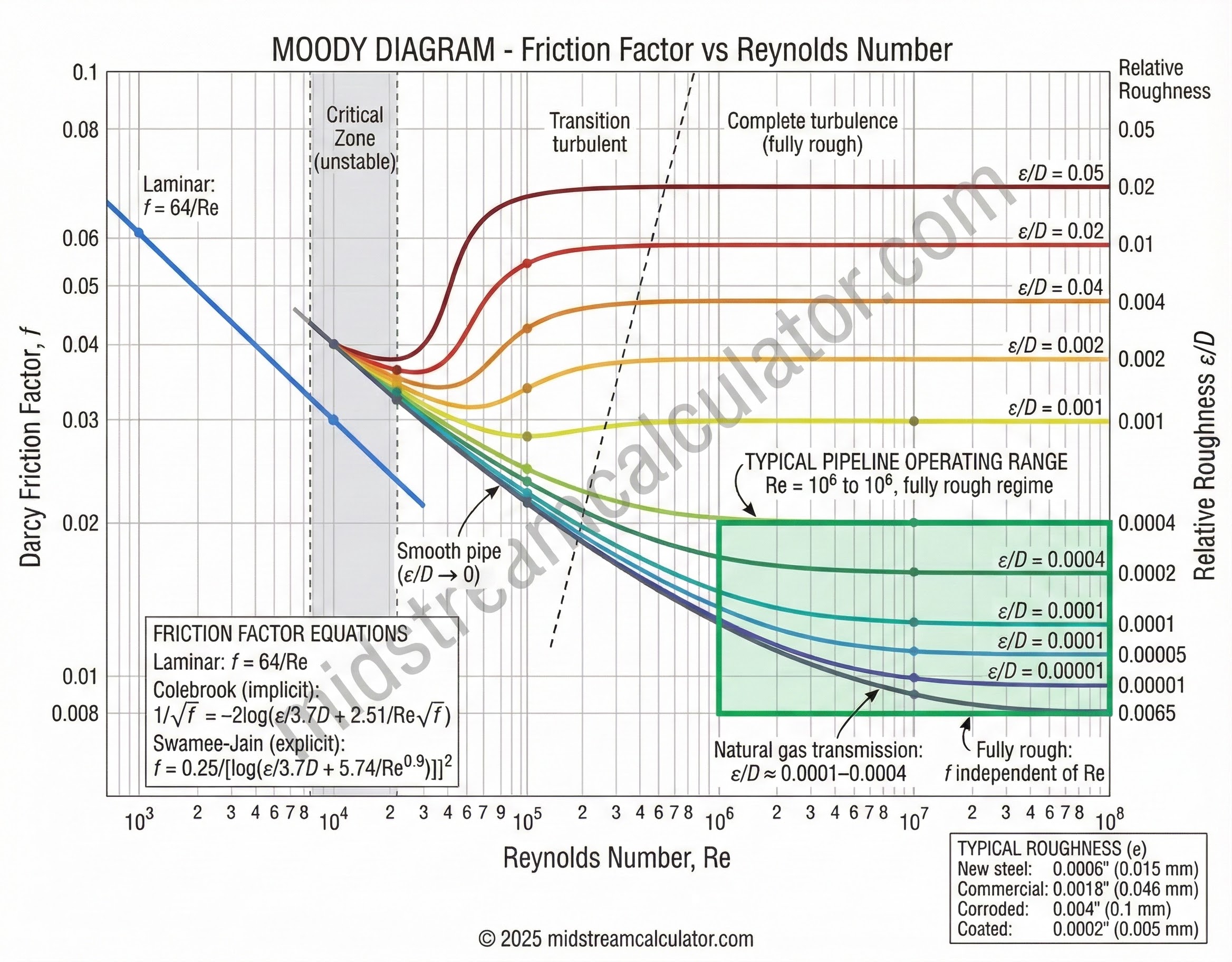
Friction factor depends on Reynolds number and pipe roughness. The AGA method uses explicit equations for different flow regimes.

Colebrook-White Equation (Implicit)

1/√f = -2 × log₁₀(ε/(3.7D) + 2.51/(Re×√f)) Where: f = Darcy friction factor ε = Absolute roughness (inches) D = Inside diameter (inches) Re = Reynolds number Requires iteration—use Swamee-Jain for direct solution.

Swamee-Jain Equation (Explicit)

f = 0.25 / [log₁₀(ε/(3.7D) + 5.74/Re^0.9)]² Direct solution, accurate within 1% of Colebrook.

Typical Pipe Roughness

Pipe Condition	ε (inches)	ε (mm)
New steel, clean	0.0006	0.015
Commercial steel	0.0018	0.046
Moderately corroded	0.004	0.1
Heavily corroded	0.02	0.5
Internally coated	0.0002–0.0004	0.005–0.01

Moody diagram with Reynolds number on the x-axis and Darcy friction factor on the y-axis showing roughness curves. — Moody diagram: friction factor vs Reynolds number with relative roughness curves and typical pipeline operating range.

Pick f

Use Swamee-Jain or Colebrook. Swamee-Jain is explicit and within 1% of Colebrook for turbulent flow.

Set ε

Choose roughness. New coated pipe ~0.0002–0.0004 in; aged lines may be 0.002–0.004 in.

Apply E

Adjust efficiency. Use a pipeline efficiency factor (E) for fittings, deposits, uncertainty.

Pipeline Efficiency

Efficiency factor E accounts for bends, fittings, deposits, and measurement uncertainty:

E = 1.0: Theoretical (new, clean, straight pipe)
E = 0.92–0.95: Typical new pipeline
E = 0.85–0.90: Aged pipeline with deposits
E = 0.80–0.85: Poor condition or many fittings

4. Elevation Effects

For pipelines with elevation change, a correction term accounts for hydrostatic head:

Elevation correction: P₂² = P₁² × e^s - (P₁² - P₂²)_friction × [(e^s - 1) / s] Where: s = 0.0375 × SG × (H₂ - H₁) / (T × Z) H₁, H₂ = Elevations at inlet and outlet (ft) Simplified (small elevation change): ΔP_elevation ≈ 0.0375 × SG × ΔH × P_avg / (T × Z)

Elevation Impact

Pipeline Profile	Effect on Capacity
Uphill (outlet higher)	Reduces capacity—gravity opposes flow
Downhill (outlet lower)	Increases capacity—gravity assists flow
Hilly terrain	Net effect depends on total elevation change

Rule of thumb: For natural gas (SG ≈ 0.65), every 100 ft elevation gain requires ~0.03 psi additional pressure at typical pipeline conditions. Significant for mountain crossings.

5. Design Considerations

Capacity Increase Options

Method	Effect	Considerations
Increase diameter	Q ∝ D^2.5 to D^2.67	Highest capital cost
Add compression	Raise P₁	Operating cost, fuel consumption
Loop pipeline	Parallel pipe reduces ΔP	Partial looping effective
Reduce delivery pressure	Lower P₂ increases ΔP	Limited by customer requirements
Internal coating	Reduce roughness	10–15% capacity gain typical

Example: Pipeline Sizing

Given: Q = 100 MMSCFD, P₁ = 1000 psia, P₂ = 600 psia, L = 50 miles, SG = 0.65, T = 520°R, Z = 0.9, E = 0.92

Using Panhandle B:

100×10⁶ = 737 × 0.92 × (520/14.73)^1.02 ×
[(1000² - 600²)/(0.65^0.961 × 520 × 50 × 0.9)]^0.51 × D^2.53

Solving: D^2.53 = 100×10⁶ / (737 × 0.92 × 35.5 × 46.8)
D^2.53 = 89.3
D = 89.3^(1/2.53) = 7.8 inches

Select: 8.625" OD pipe (8" nominal, ID ≈ 7.98")

References

GPSA Engineering Data Book, Section 17 (Fluid Flow)
AGA Report No. 3 – Orifice Metering
Crane Technical Paper 410 – Flow of Fluids
Menon, E.S. – Gas Pipeline Hydraulics