What is the difference between NPV and IRR for midstream project evaluation?

NPV calculates the present dollar value of all project cash flows at a specified discount rate, while IRR finds the discount rate that makes NPV equal to zero. NPV is preferred for comparing projects of different sizes, while IRR provides an intuitive percentage return for quick screening.

How is WACC calculated for midstream infrastructure investments?

WACC = (E/V) × Re + (D/V) × Rd × (1-T), where E is equity value, D is debt value, V is total value, Re is cost of equity, Rd is cost of debt, and T is the tax rate. Typical midstream WACC ranges from 8-12% depending on the company's capital structure and risk profile.

What is MACRS depreciation and how does it affect midstream project NPV?

MACRS (Modified Accelerated Cost Recovery System) allows front-loaded depreciation of capital assets, creating larger tax shields in early years. Midstream assets typically fall under 7-year or 15-year MACRS schedules, and the accelerated deductions improve project NPV compared to straight-line depreciation.

What sensitivity variables have the greatest impact on midstream project NPV?

The variables with the greatest NPV impact are typically throughput volume (revenue driver), commodity prices or tariff rates, capital cost overruns, operating costs, and discount rate assumptions. Sensitivity analysis should test ±20-30% variation in these key inputs to assess project robustness.

What is Net Present Value (NPV) and how is it used in midstream project evaluation?

NPV is the sum of all future cash flows discounted to present value minus the initial investment. A positive NPV indicates a project creates value above the required return rate. It is the primary metric for evaluating pipeline, compressor station, and processing plant investments.

What discount rate should be used for midstream pipeline NPV analysis?

The discount rate is typically the Weighted Average Cost of Capital (WACC), ranging from 8-12% for midstream companies. WACC accounts for the cost of both debt and equity capital. Higher-risk projects may use risk-adjusted rates 2-5% above WACC.

How does project life affect NPV for midstream infrastructure investments?

Longer project lives increase NPV because more years of positive cash flow are captured. However, distant cash flows are heavily discounted, so most NPV value comes from the first 10-15 years. Typical midstream project evaluations use 15-30 year horizons matching asset useful life.

What is the Profitability Index (PI) and when should it be used?

PI = PV of cash inflows divided by PV of cash outflows, or equivalently 1 + NPV/Initial Investment. PI > 1 means accept. PI is most useful for capital rationing - when budget is limited, rank competing projects by PI to maximize value per dollar invested.

What is the difference between simple payback and discounted payback period?

Simple payback divides the initial investment by annual cash flow, ignoring the time value of money. Discounted payback uses present-valued cash flows, producing a longer and more accurate payback period. Discounted payback accounts for the opportunity cost of capital.

What is a typical acceptable payback period for midstream infrastructure projects?

Midstream companies typically require a simple payback of 2-5 years and a discounted payback of 3-7 years, depending on risk and strategic importance. Pipeline projects with long-term contracts may accept longer paybacks, while wellhead compression typically requires payback under 2-3 years.

Why is payback period alone insufficient for investment decisions?

Payback period ignores cash flows after the payback date, does not account for the time value of money (simple payback), and cannot compare projects with different cash flow patterns. It should be used alongside NPV and IRR for comprehensive investment evaluation.

How is breakeven analysis related to payback period calculations?

Breakeven analysis determines the throughput volume, price, or utilization rate at which a project's revenues exactly equal its costs. Combined with payback analysis, it shows both when the investment is recovered and what minimum operating conditions are needed to achieve that recovery.

NPV & IRR Analysis Fundamentals

1. NPV Fundamentals

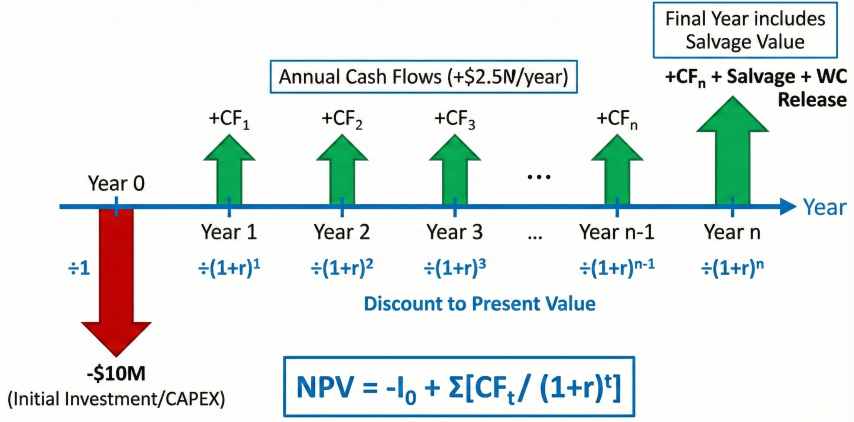
Net Present Value (NPV) is the gold standard for capital budgeting decisions. It measures the absolute dollar value a project adds to shareholder wealth by discounting all future cash flows to present value and subtracting the initial investment.

NPV Definition

Sum of discounted cash flows

Present value of all future cash flows minus initial investment.

Decision Rule

NPV > 0: Accept

Positive NPV means project creates shareholder value.

Key Advantage

Measures absolute value

Unlike IRR, NPV shows actual dollars of wealth created.

Discount Rate

WACC or hurdle rate

Use company's weighted average cost of capital.

NPV Formula

Net Present Value: NPV = -I₀ + CF₁/(1+r)¹ + CF₂/(1+r)² + ... + CFₙ/(1+r)ⁿ Or in summation notation: NPV = Σ [CFₜ / (1 + r)ᵗ] for t = 0 to n Where: I₀ = Initial investment at t=0 ($) CFₜ = Cash flow in period t ($) r = Discount rate (WACC, decimal) n = Project life (years)

NPV cash flow timeline diagram showing Year 0 initial investment as downward arrow, Years 1-n positive cash flows as upward arrows, discount factors beneath each period, and final year including salvage value and working capital release with NPV formula — NPV Cash Flow Timeline: Initial investment at Year 0, annual cash flows discounted to present value, with terminal value including salvage and working capital release.

Worked Example: Pipeline Expansion

Example: 20-mile NGL Pipeline Given: - Initial investment: $10,000,000 - Annual cash flow: $2,500,000/year for 8 years - Salvage value: $1,000,000 (Year 8) - Discount rate (WACC): 10% Solution using annuity factor: PV of annual cash flows = CF × [(1 - (1+r)⁻ⁿ) / r] PV = $2,500,000 × [(1 - 1.10⁻⁸) / 0.10] PV = $2,500,000 × 5.335 PV = $13,337,500 PV of salvage = $1,000,000 / (1.10)⁸ = $466,507 NPV = -$10,000,000 + $13,337,500 + $466,507 NPV = +$3,804,007 Decision: ACCEPT (NPV > 0)

NPV vs IRR: When They Conflict

Situation	Use NPV	Use IRR	Rationale
Mutually exclusive projects	Yes	No	NPV maximizes shareholder value; IRR can mislead
Different project sizes	Yes	No	IRR ignores scale; $50M project with 12% IRR may beat $5M project with 20% IRR
Non-conventional cash flows	Yes	No	Multiple sign changes create multiple IRRs
Single project go/no-go	Yes	Yes	Both give same accept/reject decision
Management communication	No	Yes	IRR as % is easier to communicate than NPV in $

NPV Rule: When NPV and IRR rank projects differently, always use NPV. NPV assumes cash flows are reinvested at WACC (realistic), while IRR assumes reinvestment at IRR itself (often unrealistic for high-IRR projects).

NPV Decision Framework

NPV Result	Meaning	Decision
NPV > 0	Project returns exceed cost of capital	Accept - creates shareholder value
NPV = 0	Project returns equal cost of capital	Indifferent - no value creation/destruction
NPV < 0	Project returns below cost of capital	Reject - destroys shareholder value
NPV₁ > NPV₂	Mutually exclusive projects	Select Project 1 (higher NPV)

Why NPV is preferred: NPV directly measures dollar value created, accounts for all cash flows, incorporates time value of money, and uses realistic discount rate (WACC). Superior to payback period or accounting rate of return for capital budgeting decisions.

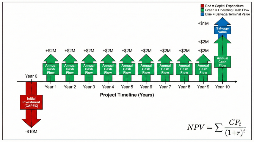
Types of Cash Flows

Project cash flow timeline showing Year 0 CAPEX outflow of -$10M in red, Years 1-10 annual operating cash flows of +$2M in green, and final year salvage value of +$1M in blue, with NPV formula displayed — Project cash flow timeline illustrating initial investment, annual operating cash flows, and terminal salvage value used in NPV calculations.

Initial investment (Year 0): Capital expenditure (CAPEX) - pipeline construction, equipment, land, permits
Operating cash flows (Years 1-N): Revenue minus operating expenses (OPEX), fuel, labor, maintenance
Terminal cash flow (Year N): Salvage value, working capital recovery, decommissioning costs
Tax effects: Depreciation tax shield, capital gains/losses on disposal

Common Pipeline Investment Types

Project Type	Typical Investment	Cash Flow Profile	Project Life
Greenfield transmission pipeline	$500M - $5B	Large upfront CAPEX, stable long-term revenue	30-50 years
Lateral extension	$10M - $100M	Moderate CAPEX, incremental revenue	20-30 years
Compressor station upgrade	$20M - $200M	CAPEX, reduced fuel costs, increased capacity	15-25 years
Integrity/replacement	$5M - $50M	CAPEX, avoided failure costs, maintained revenue	10-20 years
Metering/automation	$1M - $10M	CAPEX, reduced labor, improved accuracy	10-15 years

Discount Factor Reference Values

Present Value Factor: PV Factor = 1 / (1 + r)^t This is the present value of $1 received in year t. Example discount factors at r = 10%: Year 1: PV = 1/1.10 = 0.9091 (each dollar worth $0.91 today) Year 5: PV = 1/(1.10)^5 = 0.6209 Year 10: PV = 1/(1.10)^10 = 0.3855 Year 20: PV = 1/(1.10)^20 = 0.1486 Note: Distant cash flows heavily discounted (Year 20 dollar worth only $0.15 today)

Worked Example: 20-Mile Pipeline Lateral (Annuity Approach)

Example: 20-Mile Lateral Extension Initial investment (Year 0): - Pipeline construction: $25M - Compressor station: $10M - Land and permits: $2M Total CAPEX: I₀ = -$37M Annual cash flows (Years 1-20): - Revenue (tariff): $8M/year - Operating expenses: -$2M/year - Net annual cash flow: CF = $6M/year Discount rate: r = 10% (WACC) Salvage value (Year 20): S = $5M NPV Calculation: Method 1: Year-by-year NPV = -37 + 6/(1.10)¹ + 6/(1.10)² + ... + 6/(1.10)²⁰ + 5/(1.10)²⁰ Method 2: Annuity formula (equal cash flows) PV of annuity = CF × [(1 - (1+r)^-N) / r] PV of annuity = 6 × [(1 - 1.10^-20) / 0.10] PV of annuity = 6 × [0.8514 / 0.10] PV of annuity = 6 × 8.514 = $51.08M PV of salvage = 5 / (1.10)^20 = 5 × 0.1486 = $0.74M NPV = -37 + 51.08 + 0.74 = $14.82M IRR Calculation (find r where NPV = 0): By iteration (Excel IRR function): IRR = 15.4% Since IRR (15.4%) > WACC (10%), project exceeds cost of capital by 5.4 pp. Decision: Accept project (NPV > 0, creates $14.82M value, IRR > WACC)

Profitability Index

Profitability Index (PI): PI = PV(Cash Inflows) / PV(Cash Outflows) = 1 + NPV / Initial Investment For the 20-mile lateral example above: PI = 1 + 14.82 / 37 = 1.40 Interpretation: PV of inflows is 1.40× the initial investment; each $1 invested returns $1.40 of present value (i.e., $0.40 of NPV). Decision rule: PI > 1: Accept (equivalent to NPV > 0) PI < 1: Reject Use for capital rationing: Rank projects by PI when budget limited. PI is especially useful when comparing projects of different sizes within a fixed capital budget.

Unequal Cash Flows Example

Many midstream projects have varying cash flows over time as tariffs escalate, volumes ramp, or contracts step up:

Example: Compressor Station with Increasing Tariffs Year 0: CAPEX = -$50M Year 1-5: CF = $8M/year Year 6-10: CF = $10M/year (tariff increase) Year 11-15: CF = $12M/year Year 15: Salvage = $8M Discount rate: r = 9% Calculate NPV by summing discounted cash flows by tranche: Years 1-5: PV = 8 × [(1-1.09^-5)/0.09] = 8 × 3.8897 = $31.12M Years 6-10: PV = 10 × [(1-1.09^-5)/0.09] × (1.09)^-5 = 10 × 3.8897 × 0.6499 = $25.28M Years 11-15: PV = 12 × [(1-1.09^-5)/0.09] × (1.09)^-10 = 12 × 3.8897 × 0.4224 = $19.72M Salvage: PV = 8 / (1.09)^15 = 8 × 0.2745 = $2.20M NPV = -50 + 31.12 + 25.28 + 19.72 + 2.20 = $28.32M ✓ Project highly attractive with NPV = $28M

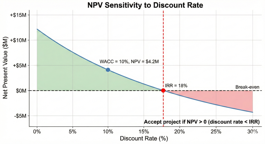
NPV profile showing how net present value decreases as discount rate increases, crossing zero at the internal rate of return (IRR = 18%).

Mid-Year Convention

For more accuracy, assume cash flows occur mid-year instead of year-end:

Mid-Year Discounting: Standard (year-end): PV = CF / (1+r)^t Mid-year: PV = CF / (1+r)^(t-0.5) Effect: Increases NPV slightly (cash received sooner) For Year 1 cash flow at 10% discount: Year-end PV: CF / 1.10 = 0.9091 × CF Mid-year PV: CF / 1.10^0.5 = CF / 1.0488 = 0.9535 × CF Difference: ~4.8% higher PV with mid-year convention Use mid-year for monthly/continuous cash flows (tariff revenue) Use year-end for annual lump sums (tax payments)

Common NPV Pitfalls

Ignoring taxes: Use after-tax cash flows; depreciation creates tax shield
Sunk costs: Exclude past expenditures (e.g., feasibility studies already paid)
Allocated overhead: Include only incremental costs caused by project
Inflation: Match nominal cash flows with nominal discount rate, or real with real
Working capital: Include working capital investment and recovery
Opportunity cost: Include forgone alternatives (e.g., land could be sold)

Tax considerations: Pipelines use MACRS depreciation (15-year or 20-year property). Depreciation is non-cash expense that reduces taxable income, creating tax shield. Tax shield value = Depreciation × Tax Rate. Must include in cash flow analysis (see Section 4).

2. IRR & MIRR Methods

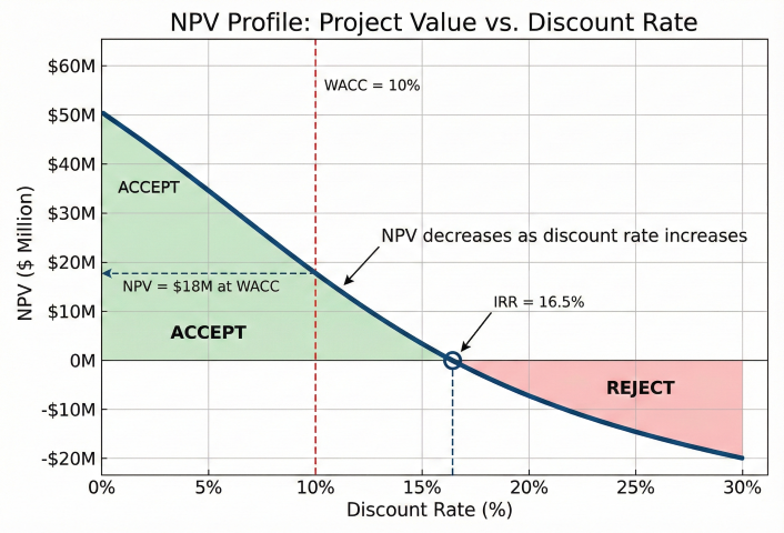
Internal Rate of Return (IRR) is the discount rate that makes NPV equal to zero. It represents the project's effective annual return. However, IRR has limitations that Modified IRR (MIRR) addresses.

IRR Formula

IRR Definition: Find r such that NPV = 0: 0 = -I₀ + CF₁/(1+IRR)¹ + CF₂/(1+IRR)² + ... + CFₙ/(1+IRR)ⁿ Decision Rules: - IRR > WACC → Accept project - IRR < WACC → Reject project - IRR = WACC → Indifferent (NPV = 0) IRR cannot be solved algebraically for n > 2. Use Newton-Raphson iteration or financial calculator.

NPV Profile Chart: NPV decreases with higher discount rates. IRR occurs where curve crosses zero. Accept projects when discount rate < IRR (NPV > 0).

Newton-Raphson Method for IRR

Iterative Solution: r(n+1) = r(n) - f(r) / f'(r) Where: f(r) = NPV(r) = Σ [CFₜ / (1+r)ᵗ] f'(r) = dNPV/dr = -Σ [t × CFₜ / (1+r)^(t+1)] Algorithm: 1. Initial guess: r₀ = 10% 2. Calculate NPV and derivative at r₀ 3. Update: r₁ = r₀ - NPV(r₀)/NPV'(r₀) 4. Repeat until |r(n+1) - r(n)| < 0.0001 Typically converges in 3-5 iterations.

Modified IRR (MIRR)

MIRR solves two IRR problems: (1) unrealistic reinvestment assumption and (2) multiple IRRs with non-conventional cash flows.

MIRR Formula: MIRR = [(FV of positive CFs / |PV of negative CFs|)^(1/n)] - 1 Where: - Positive CFs compounded forward at reinvestment rate (typically WACC) - Negative CFs discounted back at finance rate (cost of debt or WACC) FV = Σ [CFₜ × (1 + r_reinvest)^(n-t)] for CFₜ > 0 PV = Σ [|CFₜ| / (1 + r_finance)^t] for CFₜ < 0 MIRR is always unique (single solution). MIRR < IRR when IRR > reinvestment rate (typical case).

Example: IRR vs MIRR Comparison

Pipeline Project: Cash flows: CF₀ = -$10M, CF₁...₈ = $2.5M/year WACC = 10% IRR Calculation: By iteration: IRR = 18.6% MIRR Calculation (reinvest at 10%): FV of positive CFs = $2.5M × [(1.10)⁷ + (1.10)⁶ + ... + 1.0] FV = $2.5M × 11.436 = $28.59M PV of negative CF = $10M (at t=0) MIRR = ($28.59M / $10M)^(1/8) - 1 MIRR = (2.859)^0.125 - 1 MIRR = 14.0% MIRR (14.0%) < IRR (18.6%) MIRR is more realistic because it assumes reinvestment at WACC (10%), not at IRR (18.6%).

Multiple IRR Problem

Cash Flow Pattern	IRR Count	Example	Solution
Conventional (-, +, +, +)	1 unique	Standard pipeline project	Use IRR normally
Non-conventional (-, +, +, -)	0, 1, or 2+	Mining with reclamation cost	Use NPV or MIRR
All negative	None	Pure cost project	Use cost-benefit analysis

Best Practice: Many midstream companies now require both IRR and MIRR for capital approval. MIRR provides a more conservative, realistic return estimate. Use MIRR when comparing projects with different cash flow timing patterns.

3. WACC & Discount Rates

The Weighted Average Cost of Capital (WACC) represents the blended cost of all capital sources. It is the appropriate discount rate for projects of average risk. Project-specific risk adjustments may be added.

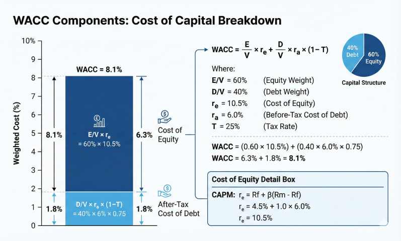
WACC Formula

Weighted Average Cost of Capital: WACC = (E/V) × rₑ + (D/V) × r_d × (1 - T_c) Where: E = Market value of equity ($) D = Market value of debt ($) V = E + D = Total firm value ($) rₑ = Cost of equity (%) r_d = Cost of debt, before tax (%) T_c = Corporate tax rate (%) (1 - T_c) = Tax shield on interest Target capital structure: E/V = Equity weight (typically 50-70% for midstream) D/V = Debt weight (typically 30-50% for midstream)

WACC components diagram showing stacked bar with cost of equity (6.3%) and after-tax cost of debt (1.8%) summing to 8.1% WACC, capital structure pie chart showing 60% equity and 40% debt, CAPM formula for cost of equity calculation — WACC Components: Weighted average of cost of equity (via CAPM) and after-tax cost of debt, reflecting target capital structure.

Cost of Equity: CAPM

Capital Asset Pricing Model: rₑ = R_f + β × (R_m - R_f) Where: rₑ = Required return on equity (%) R_f = Risk-free rate (10-yr Treasury, ~4-5%) β = Beta (systematic risk vs. market) R_m = Expected market return (~10-11%) (R_m - R_f) = Equity risk premium (~5-7%) Midstream Beta Ranges: - Interstate pipelines: β = 0.6-0.8 (low risk) - Gathering/processing: β = 1.0-1.3 (commodity exposure) - Integrated midstream MLPs: β = 0.7-1.1 Example (gathering system): R_f = 4.5%, β = 1.2, (R_m - R_f) = 6.5% rₑ = 4.5% + 1.2 × 6.5% = 12.3%

Cost of Debt

After-Tax Cost of Debt: r_d (after-tax) = r_d (before-tax) × (1 - T_c) Methods to determine before-tax r_d: 1. Yield to Maturity (YTM) on existing bonds 2. Credit spread over Treasuries based on rating 3. Recent bank loan rates Credit Spreads by Rating (over 10-yr Treasury): - AAA/AA: +0.5-1.0% - A: +1.0-1.5% - BBB: +1.5-2.5% - BB: +2.5-4.0% Example (BBB-rated company): Treasury = 4.5%, Spread = 2.0% Before-tax r_d = 6.5% Tax rate = 25% After-tax r_d = 6.5% × (1 - 0.25) = 4.9%

Complete WACC Example

Midstream Company WACC: Capital Structure: E/V = 60% equity D/V = 40% debt Cost of Equity (CAPM): R_f = 4.5%, β = 1.0, ERP = 6.0% rₑ = 4.5% + 1.0 × 6.0% = 10.5% Cost of Debt: Before-tax r_d = 6.0% Tax rate = 25% After-tax r_d = 6.0% × 0.75 = 4.5% WACC Calculation: WACC = (0.60 × 10.5%) + (0.40 × 4.5%) WACC = 6.3% + 1.8% WACC = 8.1%

Risk-Adjusted Discount Rates

Project Type	Risk Level	Adjustment	Example Rate
Replacement/maintenance	Very Low	WACC - 2%	6%
Expansion (contracted)	Low	WACC	8%
Expansion (merchant)	Medium	WACC + 2-4%	10-12%
New basin development	High	WACC + 4-6%	12-14%
International/emerging market	Very High	WACC + 6-10%	14-18%

Discount Rate Sensitivity: A 2% change in WACC can swing NPV by 20-30% for long-lived infrastructure. For a 20-year project with $100M investment and $15M/year cash flows: NPV at 8% = $47M, NPV at 10% = $28M (40% lower). Always test sensitivity to discount rate assumptions.

Typical WACC by Industry Segment

Industry Segment	Typical WACC	Risk Characteristics
Regulated pipelines (interstate)	7-9%	Low risk, stable tariffs, regulatory protection
Gathering & processing	9-11%	Moderate risk, commodity price exposure
Midstream MLPs	8-10%	Fee-based, long-term contracts
Export terminals (LNG)	10-12%	Higher risk, international exposure, large CAPEX
E&P (upstream)	12-15%	High risk, commodity price volatility

Real vs. Nominal Rates (Fisher Equation)

Fisher Equation: (1 + r_nominal) = (1 + r_real) × (1 + inflation) Or approximately: r_nominal ≈ r_real + inflation Where: r_nominal = Nominal discount rate (includes inflation) r_real = Real discount rate (inflation-adjusted) inflation = Expected inflation rate Example: If WACC = 9% nominal and inflation = 2.5% r_real = (1.09 / 1.025) - 1 = 6.34% Consistency requirement: - Nominal cash flows → use nominal discount rate - Real cash flows → use real discount rate Most corporate analyses use nominal rates and nominal cash flows.

WACC limitations: WACC assumes constant capital structure and risk over project life. For projects that change company risk profile or financing, use APV (Adjusted Present Value) method. For very long projects (30+ years), consider declining discount rate (lower rates for distant cash flows).

4. Cash Flow Analysis

Accurate cash flow forecasting is the foundation of reliable NPV/IRR analysis. Free Cash Flow to Firm (FCFF) is the appropriate measure for project evaluation.

Free Cash Flow Formula

Free Cash Flow to Firm (FCFF): FCFF = EBIT × (1 - Tax) + Depreciation - CAPEX - ΔWC Or equivalently: FCFF = Revenue - OPEX - Taxes + Depreciation × Tax - CAPEX - ΔWC Where: EBIT = Earnings before interest and taxes Tax = Marginal corporate tax rate (21% federal + state) Depreciation = Non-cash charge (creates tax shield) CAPEX = Capital expenditures ΔWC = Change in working capital (increase = outflow) Note: Interest is NOT subtracted from FCFF. WACC already accounts for financing costs.

Depreciation Tax Shield

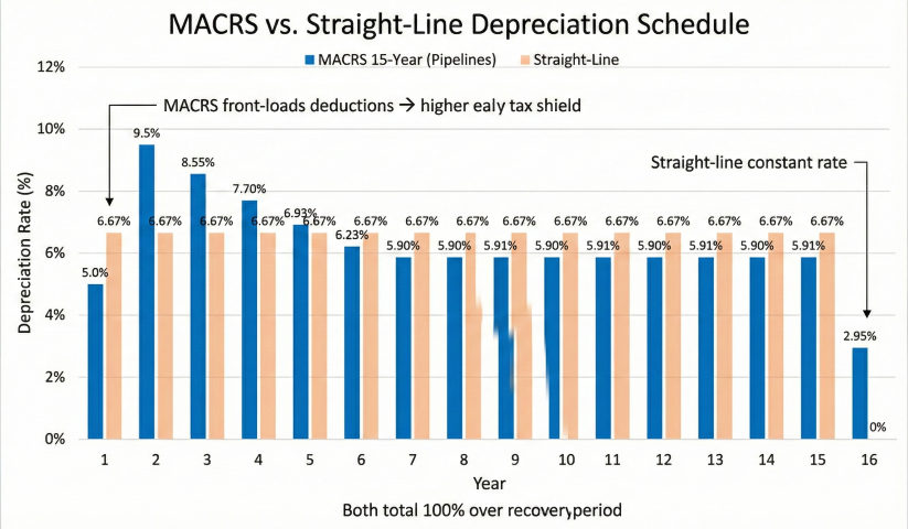
Depreciation reduces taxable income, creating a "tax shield" that increases after-tax cash flow. Accelerated depreciation (MACRS) provides higher tax shields in early years, increasing NPV.

Tax Shield Value: Annual Tax Shield = Depreciation × Tax Rate PV(Tax Shield) = Σ [Depreciationₜ × Tax Rate / (1+r)ᵗ] Depreciation Methods: 1. Straight-Line: Equal annual depreciation = Cost / Life 2. MACRS (IRS): Accelerated, front-loaded (higher early years) MACRS Classes for Midstream: - 5-Year: Vehicles, light equipment - 7-Year: Processing equipment, compressors - 15-Year: Pipelines, land improvements - 20-Year: Utility property, transmission lines

Bar chart comparing 15-year MACRS depreciation schedule for pipelines versus straight-line method, showing MACRS front-loads deductions with higher early year rates declining over time while straight-line maintains constant 6.67% annual rate — MACRS vs. Straight-Line Depreciation: MACRS front-loads deductions, providing higher tax shields in early years and increasing NPV compared to straight-line depreciation.

MACRS 15-Year Schedule (Pipelines)

Year	Rate	Year	Rate
1	5.00%	9	5.91%
2	9.50%	10	5.90%
3	8.55%	11	5.91%
4	7.70%	12	5.90%
5	6.93%	13	5.91%
6	6.23%	14	5.90%
7	5.90%	15	5.91%
8	5.90%	16	2.95%

Working Capital

Working Capital Treatment: Working Capital (WC) = Current Assets - Current Liabilities = Inventory + Receivables - Payables Year 0: WC investment = cash outflow Years 1-n: ΔWC = additional outflow if revenue grows Final Year: WC release = cash inflow (recovered at project end) Midstream WC Requirement: Typically 5-10% of annual revenue - Limited inventory (gas flows through) - Short collection cycles (monthly billing) - Long payment terms with suppliers

Terminal Value

Terminal Value Methods: 1. Salvage Value (asset-based): TV = Estimated market value at end of analysis Typical for pipelines: 20-40% of original cost Tax on gain: (Salvage - Book Value) × Tax Rate 2. Perpetuity Growth Model: TV = FCF(final) × (1 + g) / (WACC - g) g = perpetual growth rate (typically 0-2%) 3. Exit Multiple: TV = EBITDA(final) × EV/EBITDA multiple Midstream multiples: 8-12× EBITDA Terminal value often represents 30-50% of total NPV for long-lived infrastructure projects.

Cash Flow Accuracy: NPV is most sensitive to near-term cash flows due to discounting. A 10% error in Year 5 cash flow has 10× more impact than a 10% error in Year 25. Focus forecasting effort on Years 1-10; far-future cash flows can use simplified assumptions.

5. Sensitivity & Risk Analysis

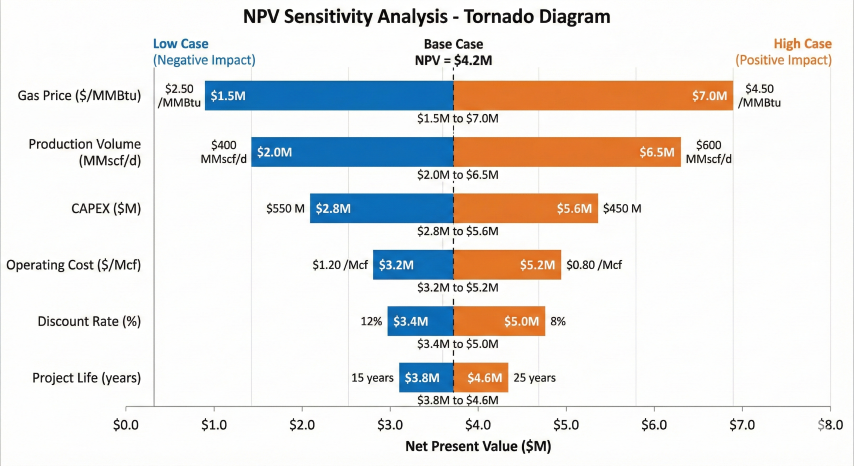
Sensitivity analysis tests how NPV/IRR change with key input variables. For midstream projects, the primary sensitivities are typically throughput volume, commodity prices (for processing plants), CAPEX, and discount rate.

One-Way Sensitivity (Tornado Chart)

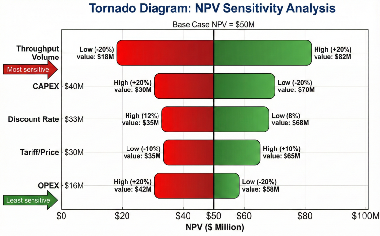
Sensitivity Analysis Process: 1. Identify key variables (typically 5-8 drivers) 2. Define range: ±10%, ±20%, or min/max bounds 3. Vary one variable, hold others at base case 4. Calculate NPV at each scenario 5. Rank by impact (tornado diagram) Example Results ($100M pipeline, base NPV = $50M): Variable | -10% | Base | +10% | Swing ------------------|---------|--------|--------|------- Throughput volume | $18M | $50M | $82M | $64M Discount rate | $68M | $50M | $35M | $33M CAPEX | $60M | $50M | $40M | $20M OPEX | $56M | $50M | $44M | $12M Ranking: Volume > Discount Rate > CAPEX > OPEX

Tornado sensitivity diagram for NPV analysis showing variables ranked by impact with throughput volume most sensitive at top, followed by CAPEX, discount rate, tariff/price, and OPEX least sensitive, with bars extending from base case NPV of $50M showing low and high scenario impacts — Tornado Sensitivity Diagram: Variables ranked by NPV impact. Throughput volume is the primary driver; OPEX has minimal effect. Red/green bars show NPV range from low to high scenarios.

Scenario Analysis

Scenario	Volume	Tariff	CAPEX	NPV	IRR
Optimistic (P10)	240 MMcf/d	$0.55	$90M	$95M	22%
Base Case (P50)	200 MMcf/d	$0.50	$100M	$50M	16%
Pessimistic (P90)	160 MMcf/d	$0.45	$110M	$8M	11%
Downside Stress	120 MMcf/d	$0.40	$120M	-$25M	7%

Breakeven Analysis

Key Breakeven Calculations: 1. Breakeven Volume (NPV = 0): Find Q such that NPV(Q) = 0 Simplified: Q_BE = [CAPEX × CRF + OPEX] / [Tariff × 365] CRF = Capital Recovery Factor = r / [1 - (1+r)^-n] 2. Breakeven Tariff (NPV = 0): Tariff_BE = [CAPEX × CRF + OPEX] / [Q × 365] 3. Maximum CAPEX (IRR = WACC): CAPEX_max = PV of all future cash flows at WACC Example: Base: Q = 200 MMcf/d, Tariff = $0.50, CAPEX = $100M WACC = 10%, n = 20 years CRF = 0.10 / [1 - 1.10^-20] = 0.1175 Annual required revenue = $100M × 0.1175 + $10M OPEX = $21.75M Breakeven Q = $21.75M / ($0.50 × 365) = 119 MMcf/d Project fails if volume < 119 MMcf/d (41% below base).

Monte Carlo Simulation

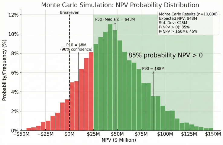
Probabilistic Analysis: Define probability distributions for uncertain variables: - Volume: Log-normal (mean 200, std dev 30 MMcf/d) - CAPEX: Triangular (min $90M, mode $100M, max $120M) - Tariff: Uniform ($0.45 to $0.55/Mcf) Run 10,000+ iterations: - Sample each variable from its distribution - Calculate NPV for each iteration - Build probability distribution of outcomes Results: - Expected NPV (mean): $48M - Standard deviation: $25M - P(NPV > 0): 85% - P(NPV > $50M): 45% - VaR (P10): NPV > $8M with 90% confidence Decision: 85% probability of positive NPV is acceptable for most corporate risk tolerances (>70% threshold).

Risk Factors by Project Type

Project Type	Primary Risk	Mitigation
Fee-based pipeline	Volume/throughput	Minimum volume commitments, anchor shipper contracts
Gas processing plant	NGL prices, plant utilization	Hedge NGL prices, long-term processing agreements
LNG terminal	Henry Hub/LNG spread, CAPEX	20-year offtake contracts, cost-reimbursable EPC
Storage facility	Storage rates, utilization	Firm storage contracts, seasonal spreads
FERC-regulated	Allowed ROE (rate case)	Regulatory precedents, prudent cost management

Industry Practice: Most midstream companies require projects to show positive NPV in both base case and pessimistic (P90) scenarios before approval. The "sanction hurdle" is typically IRR > WACC + 2-3% to provide buffer for execution risk and model uncertainty.

Worked Sensitivity Example: Pipeline Lateral

Example: 20-Mile Lateral Sensitivity Base case (from Section 1 example): - Initial investment: $37M - Annual revenue: $8M - Annual OPEX: $2M - Discount rate: 10% - Project life: 20 years - Base NPV: $14.82M Sensitivity to revenue (±20%): Revenue at $6.4M/yr (-20%): NPV = +$1.20M (ACCEPT) Revenue at $8.0M/yr (base): NPV = $14.82M Revenue at $9.6M/yr (+20%): NPV = $28.44M Sensitivity to discount rate: At 8% WACC: NPV = $21.63M At 10% WACC (base): NPV = $14.82M At 12% WACC: NPV = $9.17M At 15% WACC: NPV = $0.40M (barely positive) Critical insight: Project very sensitive to revenue; less sensitive to WACC

NPV sensitivity tornado diagram showing horizontal bars for each variable extending from base case NPV of $4.2M, with gas price having largest impact ($1.5M to $7.0M), followed by production volume, CAPEX, operating cost, discount rate, and project life — Tornado diagram ranking input variables by their impact on NPV. Gas price and production volume are the most sensitive variables requiring careful estimation.

Variable	Low Case NPV	Base NPV	High Case NPV	Range
Revenue (±20%)	$1.2M	$14.8M	$28.4M	$27.2M
Initial CAPEX (±15%)	$20.4M	$14.8M	$9.2M	$11.2M
OPEX (±25%)	$19.3M	$14.8M	$10.3M	$9.0M
Discount rate (±2%)	$21.6M	$14.8M	$9.2M	$12.4M
Project life (±5 yr)	$10.1M	$14.8M	$17.5M	$7.4M

Probability-Weighted Scenario Analysis

Three Scenario Analysis with Probabilities: Base Case (50% probability): - Revenue: $8M/yr - OPEX: $2M/yr - CAPEX: $37M - NPV: $14.82M Optimistic Case (25% probability): - Revenue: $9M/yr (higher throughput) - OPEX: $1.8M/yr (efficiency gains) - CAPEX: $35M (under budget) - NPV: $28.45M Pessimistic Case (25% probability): - Revenue: $6.5M/yr (lower throughput) - OPEX: $2.3M/yr (higher costs) - CAPEX: $40M (overrun) - NPV: -$1.23M Expected NPV: E(NPV) = 0.25 × 28.45 + 0.50 × 14.82 + 0.25 × (-1.23) E(NPV) = 7.11 + 7.41 - 0.31 = $14.21M Risk: 25% chance of negative NPV in pessimistic case

Decision Trees for Sequential Decisions

Analyze projects with decision points over time:

Example: Two-Phase Pipeline Expansion Year 0: Decide whether to build Phase 1 ($30M) Year 3: If demand high, build Phase 2 ($40M); if low, abandon Phase 1 alone: - High demand (60% prob): NPV = $20M - Low demand (40% prob): NPV = -$5M Phase 2 (if built in Year 3 after high demand): - Additional NPV = $35M (discounted to Year 3) - PV at Year 0 = 35M / (1.10)^3 = $26.3M Decision tree: Year 0: Build Phase 1 Year 3 (if high demand): Build Phase 2 Year 3 (if low demand): Do not build Phase 2 Expected NPV: E(NPV) = 0.60 × (20 + 26.3) + 0.40 × (-5) E(NPV) = 0.60 × 46.3 + 0.40 × (-5) E(NPV) = 27.78 - 2.0 = $25.78M Option value from flexibility: $25.78M vs. $11M (Phase 1 only expected NPV)

Real options: Projects with flexibility (expand, contract, abandon, delay) have option value beyond simple NPV. Use decision trees or real options analysis (Black-Scholes for deferral option) to capture value of managerial flexibility in uncertain environments.

6. Practical Applications

Capital Budgeting — Portfolio Selection

Allocate limited capital across competing projects:

Example: $100M Capital Budget, 5 Projects Available Project A: Lateral extension - CAPEX: $37M, NPV: $14.8M, IRR: 15.1%, PI: 0.40 Project B: Compressor upgrade - CAPEX: $25M, NPV: $8.2M, IRR: 14.5%, PI: 0.33 Project C: Integrity replacement - CAPEX: $15M, NPV: $3.5M, IRR: 11.8%, PI: 0.23 Project D: Metering system - CAPEX: $8M, NPV: $4.1M, IRR: 18.2%, PI: 0.51 Project E: Greenfield pipeline - CAPEX: $65M, NPV: $22.0M, IRR: 13.2%, PI: 0.34 Ranking by NPV: 1. Project E: $22.0M 2. Project A: $14.8M 3. Project B: $8.2M 4. Project D: $4.1M 5. Project C: $3.5M Total NPV if all accepted: $52.6M Total CAPEX required: $150M (exceeds $100M budget) Solution 1: Rank by NPV (accept E, A, B, D) Total CAPEX: $135M (still exceeds budget) Solution 2: Rank by PI (value per dollar invested) 1. Project D: PI = 0.51 2. Project A: PI = 0.40 3. Project E: PI = 0.34 4. Project B: PI = 0.33 5. Project C: PI = 0.23 Accept D + A + B: CAPEX = $70M, Total NPV = $27.1M ✓ Add C: CAPEX = $85M, Total NPV = $30.6M ✓ Optimal portfolio: D, A, B, C for $85M CAPEX, $30.6M NPV Remaining $15M for smaller projects or reserve

Compressor Station Economics

Example: Add Compression for Capacity Increase Current capacity: 500 MMcf/day With compressor: 650 MMcf/day (+30%) Investment: $50M compressor station Incremental revenue: - Additional throughput: 150 MMcf/day - Tariff: $0.50/Mcf - Annual revenue increase: 150,000 × 365 × $0.50 = $27.4M/yr Incremental costs: - Fuel (natural gas): 4,500 hp × 7.5 scf/hp-hr × 8760 hr × $4/Mcf = $1.18M/yr - Maintenance: $1.2M/yr - Labor: $0.5M/yr - Total OPEX: $2.88M/yr Net cash flow: $27.4M - $2.88M = $24.52M/yr NPV at 9% WACC, 20-year life: PV annuity = 24.52 × [(1 - 1.09^-20) / 0.09] = 24.52 × 9.129 = $223.8M NPV = -50 + 223.8 = $173.8M ✓ IRR: Solve 0 = -50 + 24.52/(1+IRR)^1 + ... + 24.52/(1+IRR)^20 IRR ≈ 49% (very high return) Decision: Highly attractive project, NPV = $174M, IRR = 49%

Pipeline Replacement Decision

Example: Replace vs. Repair Aging Pipeline Current situation: - 40-year-old pipeline with corrosion - Increasing leak rate, integrity concerns - Annual maintenance: $2M/yr and rising Option 1: Continue operating (do nothing) - Maintenance costs escalate: $2M yr1, $2.3M yr2, $2.6M yr3, ... - Risk of failure: 5% annual probability - Failure cost: $25M (cleanup, lost revenue, regulatory penalties) - Expected annual failure cost: 0.05 × $25M = $1.25M - Total annual cost: ~$3.5M/yr (rising) - PV of 20-year costs at 9%: $3.5M × 9.129 = $31.95M Option 2: Full replacement - New pipeline CAPEX: $60M - Annual maintenance (new): $0.5M/yr - Failure risk: 0.1% (negligible) - PV of 20-year costs: $0.5M × 9.129 = $4.56M - Total cost (PV): $60M + $4.56M = $64.56M Option 3: Partial replacement (hotspots only) - Selective replacement CAPEX: $25M - Annual maintenance: $1.2M/yr - Failure risk: 1% annual - Expected failure cost: 0.01 × $25M = $0.25M - Total annual cost: $1.45M/yr - PV: $25M + $1.45M × 9.129 = $38.24M Comparison (all costs in PV): Do nothing: $31.95M (but rising, high risk) Partial replacement: $38.24M Full replacement: $64.56M Incremental NPV (partial vs. do nothing): Cost increase: $38.24M - $31.95M = $6.29M Benefit: Reduced failure risk, regulatory compliance Decision: Partial replacement justified if compliance required Incremental NPV (full vs. partial): Cost increase: $64.56M - $38.24M = $26.32M Benefit: Very low failure risk, 40-year asset life Decision: Full replacement if long-term operation planned

Tariff Negotiation Analysis

Determine minimum acceptable tariff for pipeline project:

Required Tariff Calculation: Project: 100-mile, 24" pipeline CAPEX: $250M OPEX: $5M/year Design capacity: 500 MMcf/day Expected utilization: 70% (350 MMcf/day average) WACC: 9%, Project life: 30 years Annual throughput: 350,000 Mcf/day × 365 days = 127.75 MMcf/year Find tariff that gives NPV = 0 (break-even): 0 = -250 + (Tariff × 127.75M - 5M) × [(1-1.09^-30)/0.09] Annuity factor = 10.274 0 = -250 + (Tariff × 127.75M - 5M) × 10.274 0 = -250 + 1312.5M × Tariff - 51.4M 301.4M = 1312.5M × Tariff Tariff_breakeven = 301.4 / 1312.5 = $0.230/Mcf Add margin for acceptable return (NPV = $50M target): 50 = -250 + (Tariff × 127.75M - 5M) × 10.274 50 = (Tariff × 127.75M - 5M) × 10.274 - 250 300 = (Tariff × 127.75M - 5M) × 10.274 29.19 = Tariff × 127.75M - 5M Tariff_target = 34.19M / 127.75M = $0.268/Mcf Conclusion: Minimum tariff $0.23/Mcf (breakeven) Target tariff $0.27/Mcf for $50M NPV (20% return on investment)

Acquisition Valuation

Value existing pipeline asset for acquisition:

Example: Pipeline Acquisition Analysis Target: Existing gathering system Current revenue: $30M/year Current OPEX: $12M/year Remaining useful life: 15 years WACC: 10% Base case valuation (no improvements): Annual cash flow: $30M - $12M = $18M PV = 18M × [(1-1.10^-15)/0.10] = 18M × 7.606 = $136.9M Add terminal value (salvage): Salvage value = $20M at Year 15 PV = 20M / (1.10)^15 = 20M × 0.2394 = $4.8M Total value: $136.9M + $4.8M = $141.7M Post-acquisition improvements: - OPEX reduction (synergies): -$2M/year - Capacity expansion: +$5M/year revenue - Incremental cash flow: $7M/year PV of improvements: 7M × 7.606 = $53.2M Maximum acquisition price (with synergies): Value = $141.7M + $53.2M = $194.9M Less: Integration costs ($10M) and risk buffer (10%) Bid price: ($194.9M - $10M) × 0.90 = $166.4M Negotiation range: $140M - $165M

Common Pipeline NPV Applications

Application	Key Considerations	Typical Project Life
Greenfield transmission	Large CAPEX, long-term contracts, regulatory approvals	30-50 years
Lateral/extension	Incremental revenue, connection risk, anchor shippers	20-30 years
Compression addition	Capacity increase, fuel costs, existing system integration	20-25 years
Pipeline replacement	Avoided failure costs, regulatory compliance, salvage value	30-40 years
Metering/SCADA upgrade	Labor savings, accuracy improvement, technology obsolescence	10-15 years
Acquisition	Synergies, integration costs, due diligence risks	15-30 years remaining

Best practices: Always perform sensitivity analysis on key assumptions (tariff, throughput, CAPEX). Use probability-weighted scenarios for high-uncertainty projects. Include real options value for flexible projects (phased expansion, abandonment options). Conservative assumptions better than optimistic for capital approval.

Industry Standards and References

FERC regulations: Federal Energy Regulatory Commission tariff and rate-making guidelines for interstate pipelines
IRS Publication 946: MACRS depreciation for pipeline assets (15-year or 20-year property)
SEC guidance: Proved reserves and project valuation disclosure requirements
GAAP/IFRS: Accounting standards for capital investments and impairment testing
Project Management Institute (PMI): Economic analysis standards and best practices
AACE International: Recommended practices for capital cost estimation and economic evaluation
SPE (Society of Petroleum Engineers): Project economics standards including SPE 84218 (Newendorp Monte Carlo methods)

7. Payback Period Analysis

Payback period is the time required for cumulative cash inflows from a project to equal the initial investment. It is one of the most widely used screening tools in capital budgeting for pipeline and midstream projects. Used alongside NPV and IRR, payback metrics provide complementary insight into liquidity recovery and risk exposure.

Pipeline expansions

Capacity additions

New compressor stations, looping, diameter increases justified by throughput revenue.

Efficiency projects

Energy savings

VFDs, insulation upgrades, heat recovery systems with utility cost reduction.

Reliability improvements

Maintenance reduction

Equipment upgrades that reduce downtime and maintenance costs.

Safety & compliance

Risk mitigation

Integrity management, leak detection, safety systems justified by avoided costs.

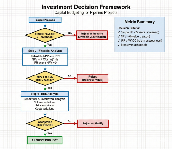
Why payback analysis matters: Simple payback provides quick go/no-go screening. Discounted payback accounts for time value of money. Combined with NPV and IRR, these metrics form a comprehensive investment decision framework.

Investment decision framework flowchart showing capital budgeting process: project proposal flows through simple payback screening, NPV and IRR financial analysis, sensitivity and risk assessment, to final approve or reject decision with metric summary showing decision criteria — Investment decision framework integrating payback period screening with NPV, IRR, and risk analysis for capital project evaluation

Advantages and Limitations of the Payback Method

Advantages:

Simplicity: Easy to calculate and explain to non-financial stakeholders
Risk indicator: Shorter payback means faster capital recovery and lower risk
Liquidity focus: Emphasizes cash recovery important for capital-constrained companies
Screening tool: Quick filter for obviously poor projects before detailed analysis

Limitations:

Ignores cash flows beyond payback: Doesn't consider project life or total profitability
No time value (simple): Simple payback doesn't discount future cash flows
Arbitrary cutoff: Payback threshold (e.g., 3 years) may not align with value creation
Biased against long-term projects: May reject valuable long-lived infrastructure

Simple Payback Period — Fundamental Equation

Simple Payback Period (Equal Annual Cash Flows): Payback Period = Initial Investment / Annual Cash Flow PP = I₀ / CF Where: PP = Payback period (years) I₀ = Initial investment ($) CF = Net annual cash flow ($/year) Example: Initial investment: $500,000 Annual cost savings: $125,000/year PP = $500,000 / $125,000 = 4.0 years

Unequal Cash Flows — Cumulative Method

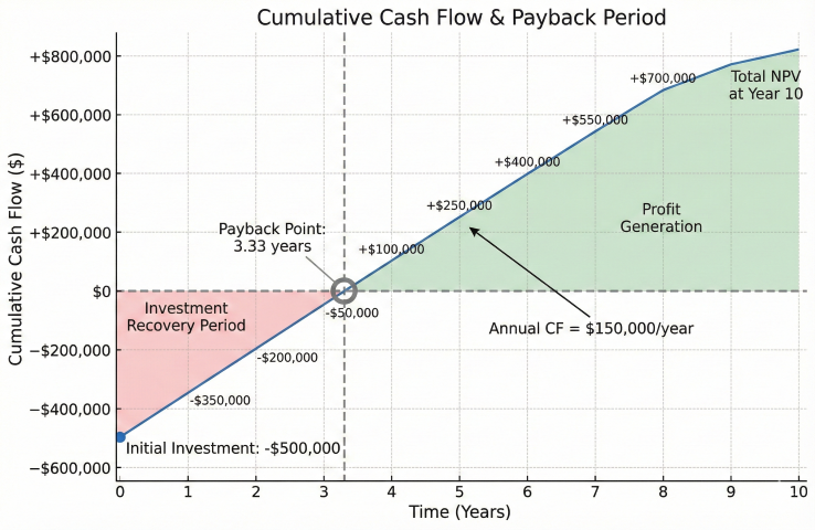
When cash flows vary by year, calculate cumulative cash flow and find when it equals initial investment:

Cumulative Cash Flow Method: Cumulative CF_n = Σ(CF₁ + CF₂ + ... + CF_n) Find n where Cumulative CF_n ≥ I₀ If recovery occurs partway through year n: PP = (n-1) + (I₀ - Cumulative CF_(n-1)) / CF_n Example with varying cash flows: Initial investment: $800,000 Year 1: $150,000 → Cumulative: $150,000 Year 2: $200,000 → Cumulative: $350,000 Year 3: $250,000 → Cumulative: $600,000 Year 4: $300,000 → Cumulative: $900,000 Recovery occurs in Year 4: Remaining after Year 3: $800,000 - $600,000 = $200,000 Fraction of Year 4: $200,000 / $300,000 = 0.67 Payback Period = 3 + 0.67 = 3.67 years

Typical Payback Thresholds by Industry

Project Type	Typical Threshold	Rationale
Energy efficiency (motors, VFDs)	2-3 years	Technology obsolescence, short economic life
Process improvements	3-5 years	Moderate risk, proven technology
Pipeline capacity expansion	4-7 years	Long-term contracts, regulated returns
New facilities (greenfield)	5-10 years	30+ year design life, strategic infrastructure
Safety/environmental compliance	Not applicable	Mandatory; justify via risk reduction, not payback
R&D / pilot projects	N/A or 1-2 years	High uncertainty; very short payback or strategic value

Pipeline Expansion Payback Example

A pipeline operator considers adding a compressor station to increase throughput from 500 MMcf/d to 650 MMcf/d.

Project Data: Compressor station cost: $12,000,000 Additional throughput: 150 MMcf/d Transportation tariff: $0.50/Mcf Operating days: 350 days/year Annual O&M cost: $1,200,000/year Annual Revenue Increase: Volume = 150,000 Mcf/day × 350 days = 52,500,000 Mcf/year Revenue = 52,500,000 × $0.50 = $26,250,000/year Net Annual Cash Flow: CF = $26,250,000 - $1,200,000 = $25,050,000/year Simple Payback: PP = $12,000,000 / $25,050,000 = 0.48 years = 5.8 months Interpretation: Very attractive project with sub-1-year payback, assuming capacity can be sold.

Energy Efficiency Payback Example (VFD Retrofit)

Replace existing fixed-speed compressor motor with VFD to reduce power consumption:

Project Data: VFD installed cost: $85,000 Current power consumption: 400 kW average Expected reduction: 15% Power cost: $0.10/kWh Operating hours: 8,000 hr/year Annual Energy Savings: kWh saved = 400 kW × 0.15 × 8,000 hr = 480,000 kWh/year Cost savings = 480,000 × $0.10 = $48,000/year Simple Payback: PP = $85,000 / $48,000 = 1.77 years Interpretation: Acceptable payback for energy efficiency. Project likely approved.

Rule of thumb: For midstream operators, simple payback < 3 years is considered excellent, 3-5 years is good, 5-7 years is marginal. Projects > 7 years require strategic justification beyond financial return.

Cumulative cash flow curve showing $500,000 initial investment recovered at 3.33 years payback point, with investment recovery period shaded red and profit generation zone shaded green, annual cash flow of $150,000 per year — Cumulative cash flow curve illustrating payback period where cumulative returns equal initial investment

Discounted Payback Period

Discounted payback period accounts for the time value of money by discounting future cash flows to present value. This provides a more conservative and financially rigorous assessment than simple payback.

Present Value Formula: PV = CF / (1 + r)ⁿ Where: PV = Present value of cash flow ($) CF = Future cash flow in year n ($) r = Discount rate (decimal) n = Year number Cumulative Present Value: Cumulative PV_n = Σ [CF_i / (1 + r)ⁱ] for i = 1 to n Find n where Cumulative PV_n ≥ I₀ Interpolation: DPP = (n-1) + [(I₀ - Cumulative PV_(n-1)) / PV_n] Where DPP = Discounted payback period (years)

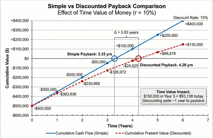
Comparison: Simple vs Discounted Payback

Project with $500,000 initial investment, 10% discount rate:

Year	Cash Flow	Cumulative CF (Simple)	PV Factor (1+0.10)ⁿ	Present Value	Cumulative PV (Discounted)
0	-$500,000	-$500,000	1.000	-$500,000	-$500,000
1	$150,000	-$350,000	1.100	$136,364	-$363,636
2	$150,000	-$200,000	1.210	$123,967	-$239,669
3	$150,000	-$50,000	1.331	$112,697	-$126,972
4	$150,000	$100,000	1.464	$102,452	-$24,520
5	$150,000	$250,000	1.611	$93,138	$68,618

Simple Payback Calculation: Recovery in Year 4: 3 + ($50,000 / $150,000) = 3.33 years Discounted Payback Calculation: Recovery in Year 5: 4 + ($24,520 / $93,138) = 4.26 years Difference: 4.26 - 3.33 = 0.93 years longer Interpretation: Discounting increases payback by ~1 year due to time value of money. The $150,000 received in Year 5 is worth only $93,138 today.

Selecting the Discount Rate for Payback

Discount Rate Type	Typical Range	When to Use
WACC (Weighted Average Cost of Capital)	8-12%	Standard projects with average risk profile
Hurdle rate (WACC + risk premium)	12-18%	High-risk projects, new technologies, uncertain markets
Cost of debt	4-8%	Debt-financed projects (not recommended; doesn't reflect equity cost)
Risk-free rate + equity premium	6-10%	Low-risk regulated utility projects
Opportunity cost	Varies	Return from next-best alternative investment

Alternative WACC Calculation Example (60/40 Capital Structure with Different Numbers)

Weighted Average Cost of Capital — Alternative Example: WACC = (E/V) × Re + (D/V) × Rd × (1 - Tc) Equity: $100M at 12% cost Debt: $40M at 6% cost Tax rate: 25% E/V = $100M / $140M = 71.4% D/V = $40M / $140M = 28.6% WACC = 0.714 × 12% + 0.286 × 6% × (1 - 0.25) WACC = 8.57% + 1.29% = 9.86% ≈ 10%

Impact of discount rate on payback: Higher discount rates penalize distant cash flows more heavily, increasing discounted payback period. A 5% increase in discount rate typically adds 0.5-1.5 years to payback for 5-10 year projects.

Comparison chart of simple payback (3.33 years) versus discounted payback (4.26 years) at 10% discount rate, showing cumulative cash flow and cumulative present value curves with time value impact annotation — Simple vs discounted payback comparison showing how time value of money extends payback period by approximately one year at 10% discount rate

When Projects Never Pay Back

Some projects have negative NPV and never achieve discounted payback:

Example of No Payback: Initial investment: $1,000,000 Annual cash flow: $80,000/year for 20 years Discount rate: 12% PV of cash flows = $80,000 × [PV annuity factor, 12%, 20 years] PV = $80,000 × 7.469 = $597,520 Since $597,520 < $1,000,000, project never pays back in PV terms. NPV = -$1,000,000 + $597,520 = -$402,480 (reject project)

Payback-Based Breakeven Throughput

For capacity expansion projects, calculate minimum volume needed to recover investment within a target payback:

Breakeven Volume Calculation: Total Annual Cost = (I₀ / PP) + Annual O&M Required Volume = Total Annual Cost / Unit Margin Where: I₀ = Initial investment PP = Target payback period (years) Unit Margin = Tariff revenue per unit - variable cost per unit Example - Pipeline Looping: Investment: $25,000,000 Target payback: 5 years Annual O&M: $800,000/year Tariff: $0.75/Mcf Variable cost: $0.05/Mcf Annual cost to recover = $25,000,000 / 5 + $800,000 = $5,800,000 Unit margin = $0.75 - $0.05 = $0.70/Mcf Breakeven volume = $5,800,000 / $0.70 = 8,285,714 Mcf/year = 22,710 Mcf/day (assuming 365 days) If project adds 200 MMcf/d capacity and can sell 25 MMcf/d or more, project exceeds breakeven requirement.

Payback-Based Breakeven Tariff

Breakeven Tariff Formula: Required Annual Revenue = (I₀ / PP) + Annual O&M Breakeven Tariff = Required Revenue / Annual Volume Example - NGL Pipeline: Investment: $150,000,000 Target payback: 7 years Annual O&M: $8,000,000/year Expected volume: 100,000 bbl/day × 350 days = 35,000,000 bbl/year Required annual revenue = $150,000,000 / 7 + $8,000,000 = $29,428,571 Breakeven tariff = $29,428,571 / 35,000,000 = $0.84/bbl If market tariff is $1.25/bbl, project has comfortable margin above breakeven.

Payback Sensitivity Analysis

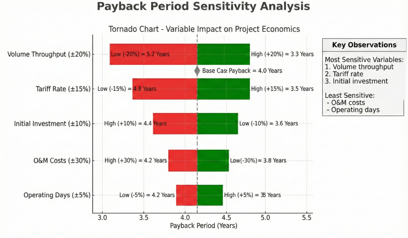
Six-scenario sensitivity table evaluating how payback period changes with key variables:

Scenario	Volume (MMcf/d)	Tariff ($/Mcf)	O&M ($/yr)	Annual CF	Payback (yrs)
Base Case	50	$0.80	$2.0M	$12.6M	3.97
Low volume (-20%)	40	$0.80	$2.0M	$9.68M	5.17
Low tariff (-15%)	50	$0.68	$2.0M	$10.41M	4.80
High O&M (+30%)	50	$0.80	$2.6M	$12.0M	4.17
Optimistic (all favorable)	60	$0.90	$1.8M	$17.91M	2.79
Pessimistic (all unfavorable)	40	$0.68	$2.6M	$7.33M	6.83

Assumes $50M investment, 365 operating days/year

Monte Carlo Simulation for Payback Risk Assessment

For high-value projects, use probabilistic analysis to quantify payback period uncertainty:

Monte Carlo Approach for Payback: 1. Define probability distributions for uncertain variables: - Volume: Normal distribution, mean 50 MMcf/d, std dev 8 MMcf/d - Tariff: Triangular distribution, min $0.65, most likely $0.80, max $0.95 - O&M: Log-normal distribution, mean $2.0M, std dev $0.4M 2. Run 10,000 simulations, randomly sampling from distributions 3. Calculate payback period for each simulation 4. Analyze results: - P10 (10th percentile): 3.1 years (optimistic) - P50 (median): 4.2 years (expected) - P90 (90th percentile): 6.8 years (pessimistic) - Probability of payback < 5 years: 72% 5. Decision: Accept if P90 < management threshold (e.g., 7 years)

Tornado chart showing payback period sensitivity analysis with volume throughput as most sensitive variable, followed by tariff rate, initial investment, O&M costs, and operating days, centered on 4.0 year base case — Sensitivity tornado chart identifying volume throughput and tariff rate as the most critical variables affecting payback period

Comparison of Investment Decision Metrics

Metric	Advantages	Disadvantages	Best Use
Simple Payback	Easy to calculate; intuitive; emphasizes liquidity	Ignores time value of money; ignores cash flows after payback	Initial screening; capital-constrained environments
Discounted Payback	Accounts for time value; conservative measure	Still ignores post-payback cash flows; arbitrary cutoff	Risk assessment; projects with uncertain long-term cash flows
NPV	Theoretically sound; accounts for all cash flows; additive	Requires accurate discount rate; not intuitive for non-finance	Primary decision criterion; ranking mutually exclusive projects
IRR	Percentage return easy to understand; no discount rate needed	Multiple IRRs possible; scale-insensitive; reinvestment assumption	Communicate returns to management; compare to hurdle rates
Profitability Index	Measures value per dollar invested; good for capital rationing	Doesn't show absolute value; can conflict with NPV	Budget constraints; ranking projects with different scales

Integrated Decision Framework — 5 Sample Projects

Comprehensive project evaluation using multiple criteria side-by-side:

Project	Investment	Simple PP	Disc. PP	NPV @10%	IRR	PI	Decision
Compressor station	$8M	3.2 yr	4.1 yr	$3.5M	18.2%	1.44	Accept - All metrics favorable
VFD retrofit	$250K	2.8 yr	3.4 yr	$75K	24.5%	1.30	Accept - Excellent returns
Pipeline looping	$40M	6.5 yr	8.9 yr	$2.1M	11.8%	1.05	Marginal - Low but positive NPV
Meter upgrades	$1.2M	8.1 yr	Never	-$350K	7.2%	0.71	Reject - NPV < 0, IRR < WACC
SCADA system	$3M	N/A	N/A	-$1.2M	N/A	N/A	Accept - Safety/reliability, not financial

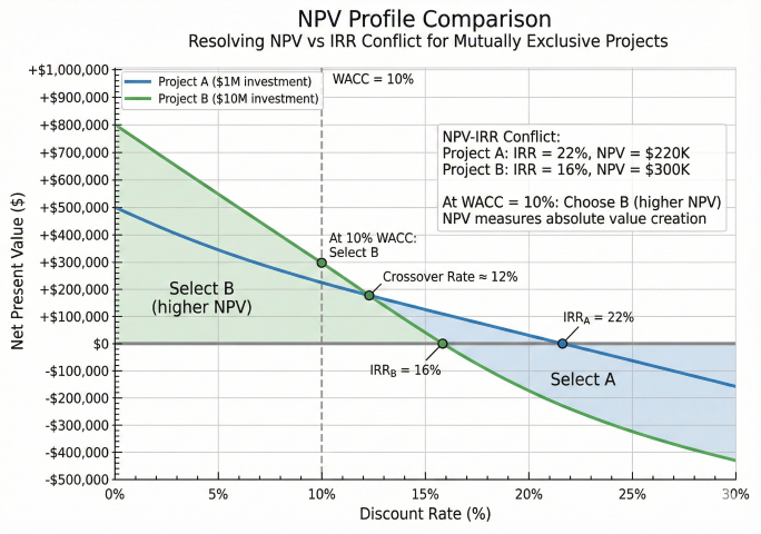
NPV vs IRR Scale Conflict — Worked Example

For mutually exclusive projects of different scales, NPV and IRR can give conflicting rankings:

Example of NPV-IRR Conflict: Project A (Small): Investment: $1,000,000 NPV: $400,000 IRR: 22% Project B (Large): Investment: $10,000,000 NPV: $2,500,000 IRR: 16% Analysis: - By IRR: Select Project A (22% > 16%) - By NPV: Select Project B ($2.5M > $0.4M) Correct Decision: Select Project B NPV measures absolute value creation. Project B adds $2.5M vs. $0.4M. Even though A has higher percentage return, B creates more shareholder value. When to use IRR: Comparing projects of similar scale and timing. When to use NPV: Mutually exclusive projects of different scales (use NPV).

NPV profile crossover chart demonstrating how NPV and IRR can give conflicting rankings for mutually exclusive projects of different scales

Decision Tree for Project Approval (4-Step Process)

Recommended Decision Process: Step 1: Calculate Simple Payback - If PP > 10 years → Likely reject (unless strategic) - If PP ≤ 3 years → Proceed to Step 2 (strong candidate) - If 3 < PP ≤ 10 → Proceed to Step 2 (requires detailed analysis) Step 2: Calculate NPV and IRR - If NPV > 0 AND IRR > WACC → Accept - If NPV < 0 OR IRR < WACC → Reject - If NPV ≈ 0 → Sensitivity analysis required Step 3: Sensitivity and Risk Analysis - Identify key uncertainties (volume, price, costs) - Calculate breakeven values - Assess probability of achieving targets - Consider strategic value, competitive position, regulatory factors Step 4: Management Review - Present all metrics with sensitivity cases - Recommend accept/reject with rationale - Identify key assumptions and risks - Propose monitoring metrics for post-approval tracking

Best practice for combined metrics: Use simple payback for initial screening, NPV as primary decision criterion, IRR for communication to management, and discounted payback for risk assessment. No single metric tells the complete story.

NPV & IRR Analysis: Project Economics Engineering Guide

NPV > 0, IRR > WACC

8-14%

3-7 years

Contents

Use this guide when you need to: