Convert between Fahrenheit, Celsius, Kelvin, and Rankine temperature scales, understand absolute vs. relative temperature for thermodynamic calculations, calculate thermal expansion, and apply correct temperature bases in process design.
Apply absolute temperature in thermodynamic equations.
Calculate thermal expansion and contraction.
1. Temperature Scales Overview
Temperature is a measure of thermal energy. Four temperature scales are used in engineering: Fahrenheit and Celsius (relative scales with arbitrary zero points), and Kelvin and Rankine (absolute scales with zero at absolute zero).
Thermodynamic calculations
Gas law equations
PV=nRT and related equations require absolute temperature (Kelvin or Rankine).
Heat transfer
Temperature differences
ΔT calculations use any scale; thermal conductivity and expansion use absolute.
Material properties
Temperature-dependent
Density, viscosity, thermal expansion vary with temperature; correct scale essential.
Fahrenheit (1724): Daniel Gabriel Fahrenheit set 0°F as temperature of equal parts ice, water, and ammonium chloride; 96°F as human body temperature (later adjusted)
Celsius (1742): Anders Celsius defined 0°C at water freezing, 100°C at boiling (1 atm); originally inverted (0 = boiling, 100 = freezing)
Kelvin (1848): William Thomson (Lord Kelvin) proposed absolute scale based on thermodynamic principles; zero is theoretical point where molecular motion ceases
Rankine (1859): William Rankine developed absolute scale using Fahrenheit degree intervals, starting at absolute zero
Scale Relationships
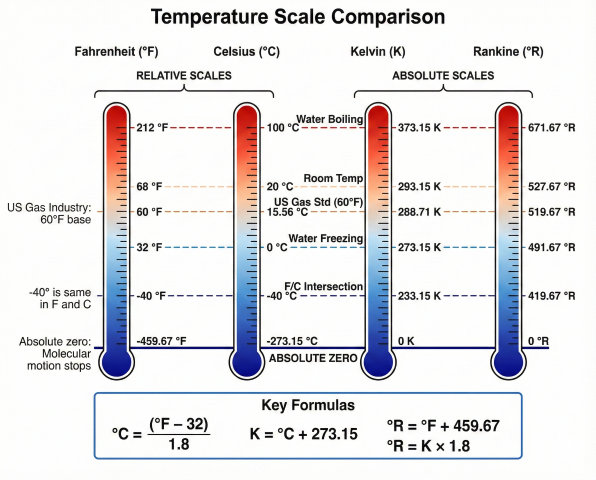
Figure 1: Four temperature scales with key reference points and conversion formulas
Degree Size Comparison:
Fahrenheit and Rankine:
- 180 degrees between water freezing and boiling
- 1°F = 1°R (same degree size)
Celsius and Kelvin:
- 100 degrees between water freezing and boiling
- 1°C = 1 K (same degree size)
Fahrenheit vs. Celsius:
- 180°F span = 100°C span
- 1°F = 5/9°C = 0.556°C
- 1°C = 9/5°F = 1.8°F
Key Reference Points:
Absolute zero:
- 0 K = 0°R = -273.15°C = -459.67°F
Water triple point (273.16 K by definition):
- 273.16 K = 0.01°C = 32.018°F = 491.688°R
Standard temperature (various definitions):
- 0°C = 32°F = 273.15 K = 491.67°R (IUPAC)
- 15°C = 59°F = 288.15 K = 518.67°R (petroleum industry)
- 20°C = 68°F = 293.15 K = 527.67°R (ambient conditions)
- 60°F = 15.56°C = 288.71 K = 519.67°R (US gas industry base)
Why temperature scale matters: Using °F instead of °R in ideal gas law PV=nRT causes 46% error at 100°F (560°R vs. 100). Similarly, confusing Celsius and Fahrenheit when reading thermocouples leads to process upsets, equipment damage, or safety incidents. In 1999, Mars Climate Orbiter was lost because contractor used Imperial units (lb-force) while NASA used SI (Newtons)—a $125M lesson in unit consistency.
2. Conversion Formulas
Accurate conversion between temperature scales requires understanding whether converting absolute temperature or temperature difference.
Fahrenheit ⇔ Celsius
Fahrenheit to Celsius:
°C = (°F - 32) × 5/9
Or equivalently:
°C = (°F - 32) / 1.8
Celsius to Fahrenheit:
°F = (°C × 9/5) + 32
Or equivalently:
°F = (°C × 1.8) + 32
Examples:
Convert 100°F to Celsius:
°C = (100 - 32) × 5/9 = 68 × 5/9 = 37.78°C
Convert 25°C to Fahrenheit:
°F = (25 × 1.8) + 32 = 45 + 32 = 77°F
Convert -40°F to Celsius:
°C = (-40 - 32) × 5/9 = -72 × 5/9 = -40°C
Note: -40°F = -40°C is the only temperature where Fahrenheit and Celsius scales intersect.
Absolute Temperature Conversions
Celsius ⇔ Kelvin:
K = °C + 273.15
°C = K - 273.15
Example:
20°C = 20 + 273.15 = 293.15 K
300 K = 300 - 273.15 = 26.85°C
Fahrenheit ⇔ Rankine:
°R = °F + 459.67
°F = °R - 459.67
Example:
70°F = 70 + 459.67 = 529.67°R
600°R = 600 - 459.67 = 140.33°F
Kelvin ⇔ Rankine:
°R = K × 9/5
K = °R × 5/9
Or:
°R = K × 1.8
K = °R / 1.8
Example:
300 K = 300 × 1.8 = 540°R
540°R = 540 / 1.8 = 300 K
Direct Fahrenheit ⇔ Kelvin:
K = (°F + 459.67) × 5/9
°F = (K × 9/5) - 459.67
Example:
100°F = (100 + 459.67) × 5/9 = 559.67 × 5/9 = 310.93 K
300 K = (300 × 1.8) - 459.67 = 540 - 459.67 = 80.33°F
Temperature Difference Conversions
When converting temperature differences (ΔT), NOT absolute temperatures, the offset terms (32, 273.15, 459.67) cancel out:
Temperature Difference (ΔT) Conversions:
ΔT(°C) = ΔT(°F) × 5/9 = ΔT(°F) / 1.8
ΔT(°F) = ΔT(°C) × 9/5 = ΔT(°C) × 1.8
ΔT(K) = ΔT(°C) [same degree size]
ΔT(°R) = ΔT(°F) [same degree size]
ΔT(K) = ΔT(°R) / 1.8
ΔT(°R) = ΔT(K) × 1.8
Example:
A process requires heating gas from 60°F to 120°F.
Temperature rise in Fahrenheit:
ΔT = 120 - 60 = 60°F
Temperature rise in Celsius:
ΔT = 60 / 1.8 = 33.33°C
Verify by converting endpoints:
60°F = 15.56°C
120°F = 48.89°C
ΔT = 48.89 - 15.56 = 33.33°C ✓
Temperature rise in Rankine:
ΔT = 60°R (same as 60°F for difference)
Temperature rise in Kelvin:
ΔT = 33.33 K (same as 33.33°C for difference)
Quick Approximation Methods
Approximation
Accuracy
Use Case
°F ≈ 2 × °C + 30
±5°F (range 0-40°C)
Quick mental conversion for ambient temperatures
°C ≈ (°F - 30) / 2
±3°C (range 32-100°F)
Reverse quick estimate
K ≈ °C + 273
±0.15 K
Engineering calculations (0.15 K error negligible in most cases)
°R ≈ °F + 460
±0.67°R
Engineering calculations (0.67°R error < 0.15%)
Common Conversion Errors
Using °F in place of °R: Forgetting to add 459.67 when absolute temperature required (ideal gas law, thermodynamic ratios)
Using °C in place of K: Forgetting to add 273.15; less obvious error than °F/°R due to smaller offset
Converting ΔT with offset: Applying +32 or +273.15 when converting temperature difference (incorrect)
Mixing scales in calculations: Using °F in equations calibrated for °C (e.g., vapor pressure correlations)
Confusing K and °K: Kelvin unit symbol is "K" without degree sign (°K is obsolete)
Comprehensive Conversion Table
Fahrenheit (°F)
Celsius (°C)
Kelvin (K)
Rankine (°R)
Reference
-459.67
-273.15
0
0
Absolute zero
-40
-40
233.15
419.67
F/C intersection
0
-17.78
255.37
459.67
Fahrenheit zero
32
0
273.15
491.67
Water freezing
60
15.56
288.71
519.67
US gas base
68
20
293.15
527.67
Room temperature
98.6
37
310.15
558.27
Human body
212
100
373.15
671.67
Water boiling
392
200
473.15
851.67
Glycol reboiler
1000
537.78
810.93
1459.67
Furnace exhaust
3. Absolute vs. Relative Temperature
Absolute temperature scales (Kelvin, Rankine) have zero at absolute zero, where molecular motion theoretically ceases. Relative scales (Celsius, Fahrenheit) have arbitrary zero points.
When to Use Absolute Temperature
Thermodynamic Calculations Requiring Absolute Temperature:
1. Ideal Gas Law:
PV = nRT
Where T MUST be in K or °R (not °C or °F)
2. Real Gas Equations (compressibility):
Reduced temperature: T_r = T / T_c
Where T and T_c both in absolute scale
3. Charles's Law:
V₁/T₁ = V₂/T₂
Where T₁, T₂ in absolute scale
4. Thermal Efficiency (Carnot cycle):
η = 1 - (T_cold / T_hot)
Where T_cold, T_hot in absolute scale
5. Radiation Heat Transfer:
Q = σ × A × (T₁⁴ - T₂⁴)
Where T in absolute scale (Stefan-Boltzmann law)
6. Acoustic Velocity in Gas:
a = √(k × R × T)
Where T in absolute scale
7. Gas Density:
ρ = (P × MW) / (R × T)
Where T in absolute scale
Common Error Example:
Incorrect (using °F instead of °R):
ρ = (1000 psia × 19 lb/lbmol) / (10.73 psia·ft³/lbmol·°R × 100°F)
ρ = 19,000 / 1,073 = 17.7 lb/ft³ ✗ (way too high!)
Correct (using °R):
T = 100°F + 459.67 = 559.67°R
ρ = (1000 × 19) / (10.73 × 559.67) = 19,000 / 6,005 = 3.16 lb/ft³ ✓
Error factor: 17.7 / 3.16 = 5.6× (560% error!)
When Relative Temperature is Acceptable
Temperature differences (ΔT) and many empirical correlations can use relative scales:
Heat transfer rate (Fourier's law): Q = k × A × ΔT / L — ΔT can be in any scale
Newton's law of cooling: Q = h × A × ΔT — ΔT can be in any scale
Specific heat calculations: Q = m × C_p × ΔT — ΔT can be in any scale (if C_p units consistent)
Empirical correlations: Many property correlations (viscosity, density, vapor pressure) use °C or °F if correlation was developed in that scale
Temperature measurement and display: Process control, temperature indicators typically use °F or °C (easier for operators)
Absolute Zero and the Third Law of Thermodynamics
Absolute Zero (0 K = 0°R):
Definition: Temperature at which entropy of perfect crystal reaches minimum (zero).
Physical meaning:
- All molecular translational motion ceases (classically)
- Quantum zero-point energy remains (quantum mechanically)
- Entropy S → 0 as T → 0 (Third Law of Thermodynamics)
Experimental approach:
- Coldest temperature achieved: ~0.00000001 K (10⁻⁸ K, 100 nanokelvin)
- Achieved using laser cooling and magnetic trapping
- Impossible to reach exactly 0 K (Third Law implication)
Engineering relevance:
- Cryogenic processes (LNG at 111 K = -162°C = -259°F)
- Superconductivity (critical temperature 0-130 K for high-T superconductors)
- Gas liquefaction requires approach to 80-120 K
Temperature Ratios and Dimensionless Groups
Dimensionless temperature ratios appear in heat transfer and thermodynamics:
Parameter
Definition
Temperature Scale Required
Reduced temperature (T_r)
T_r = T / T_c
Absolute (K or °R)
Carnot efficiency (η)
η = 1 - T_cold / T_hot
Absolute (K or °R)
Temperature rise ratio
θ = (T - T_in) / (T_out - T_in)
Any scale (cancels in difference)
Dimensionless temperature (Fourier number)
Fo = α × t / L²
N/A (time/length only)
Example: Compressor Discharge Temperature
Adiabatic Compression Temperature Rise:
T₂ / T₁ = (P₂ / P₁)^[(k-1)/k]
Where:
T₁, T₂ = Inlet and outlet temperature (absolute scale required)
P₁, P₂ = Inlet and outlet pressure (absolute)
k = Specific heat ratio (C_p / C_v ≈ 1.27 for natural gas)
Example: Compress natural gas
Inlet: T₁ = 80°F = 539.67°R, P₁ = 500 psia
Outlet: P₂ = 1500 psia
k = 1.27
Compression ratio: r = 1500 / 500 = 3.0
T₂ / T₁ = 3.0^[(1.27-1)/1.27] = 3.0^0.2126 = 1.246
T₂ = 539.67 × 1.246 = 672.4°R
Convert to Fahrenheit:
T₂ = 672.4 - 459.67 = 212.7°F
Temperature rise:
ΔT = 212.7 - 80 = 132.7°F (or 73.7°C)
Common error (using °F instead of °R):
If someone incorrectly uses T₁ = 80°F directly:
T₂ = 80 × 1.246 = 99.7°F ✗
This predicts only 19.7°F rise—grossly underestimates actual 132.7°F rise!
4. Thermal Expansion Applications
Materials expand when heated, contract when cooled. Thermal expansion calculations require correct temperature scale and coefficient units.
Linear Thermal Expansion
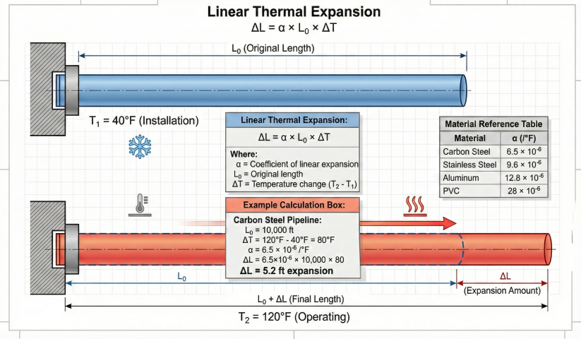
Figure 2: Linear thermal expansion showing cold-to-hot pipe growth with ΔL = α × L₀ × ΔT
Linear Expansion Formula:
ΔL = α × L₀ × ΔT
Where:
ΔL = Change in length (in, ft, mm, m)
α = Coefficient of linear thermal expansion (in/in/°F, m/m/°C, or per °F, per °C)
L₀ = Original length at reference temperature
ΔT = Temperature change (°F, °C, K, or °R)
Units of α:
- US/Imperial: in/in/°F or 1/°F (same for °R since ΔT°F = ΔT°R)
- SI/Metric: m/m/°C or 1/°C (same for K since ΔT°C = ΔTK)
Conversion: α(1/°F) = α(1/°C) / 1.8
Typical values of α:
Carbon steel: α = 6.5 × 10⁻⁶ /°F (11.7 × 10⁻⁶ /°C)
Stainless steel 304: α = 9.6 × 10⁻⁶ /°F (17.3 × 10⁻⁶ /°C)
Aluminum: α = 12.8 × 10⁻⁶ /°F (23.1 × 10⁻⁶ /°C)
Copper: α = 9.2 × 10⁻⁶ /°F (16.6 × 10⁻⁶ /°C)
PVC plastic: α = 28 × 10⁻⁶ /°F (50 × 10⁻⁶ /°C)
Concrete: α = 5-6 × 10⁻⁶ /°F (9-11 × 10⁻⁶ /°C)
Higher α → more expansion per degree temperature change
Pipeline Thermal Expansion Example
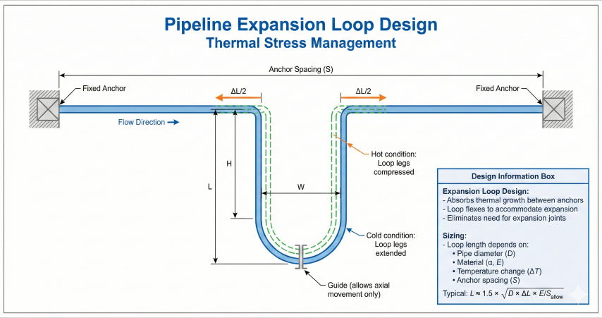
Figure 3: Pipeline expansion loop (U-bend) design for thermal stress management between anchor points
Example: Natural gas pipeline expansion
Pipeline: Carbon steel, 10,000 ft long
Installation temperature: 40°F (winter)
Operating temperature: 120°F (summer, hot gas)
Temperature change: ΔT = 120 - 40 = 80°F
α for carbon steel: 6.5 × 10⁻⁶ /°F
ΔL = α × L₀ × ΔT
ΔL = 6.5 × 10⁻⁶ × 10,000 ft × 80°F
ΔL = 0.0000065 × 10,000 × 80
ΔL = 5.2 ft
Pipeline expands 5.2 feet over 10,000 ft length (0.052% strain).
Design considerations:
- Expansion loops or bends accommodate growth (no stress buildup)
- Fixed anchor points must resist thermal loads
- Buried pipe: soil restraint creates compressive stress
- Thermal stress if constrained: σ = E × α × ΔT
For constrained carbon steel pipe (E = 29 × 10⁶ psi):
σ = 29 × 10⁶ × 6.5 × 10⁻⁶ × 80 = 15,080 psi (compressive)
This is 30% of yield strength (SMYS = 52,000 psi for X52)—significant!
Volumetric Thermal Expansion
Volume Expansion (Liquids):
ΔV / V₀ = β × ΔT
Where:
β = Coefficient of volumetric expansion (1/°F or 1/°C)
For isotropic solids: β ≈ 3α
For liquids: β is empirically determined
Typical β values (liquids):
Water (at 60°F): β = 1.1 × 10⁻⁴ /°F (2.0 × 10⁻⁴ /°C)
Gasoline: β = 7.0 × 10⁻⁴ /°F (1.26 × 10⁻³ /°C)
Diesel fuel: β = 5.0 × 10⁻⁴ /°F (9.0 × 10⁻⁴ /°C)
Crude oil (light): β = 5-6 × 10⁻⁴ /°F (9-11 × 10⁻⁴ /°C)
Methanol: β = 6.6 × 10⁻⁴ /°F (1.19 × 10⁻³ /°C)
Example: Tank truck thermal expansion
Gasoline tank: 9,000 gallons at 60°F
Temperature rise: 60°F to 100°F (ΔT = 40°F)
β for gasoline: 7.0 × 10⁻⁴ /°F
ΔV = V₀ × β × ΔT = 9,000 × 7.0 × 10⁻⁴ × 40
ΔV = 9,000 × 0.028 = 252 gallons
Gasoline expands by 252 gallons (2.8% volume increase).
If tank filled to 100% at 60°F, expansion at 100°F causes 252 gallon overflow!
This is why tank trucks have 2-5% outage (vapor space) requirement.
Safe fill at 60°F: 9,000 × 0.97 = 8,730 gallons
At 100°F: 8,730 × 1.028 = 8,974 gallons < 9,000 capacity ✓
Temperature Corrections for Liquid Volume
Custody transfer of petroleum products requires volume correction to standard temperature:
API MPMS Chapter 11 Volume Correction:
V_std = V_obs × CTL
Where:
V_std = Volume at standard temperature (60°F or 15°C)
V_obs = Observed volume at measured temperature
CTL = Correction for Temperature and pressure on Liquid
CTL ≈ 1 - β × (T_obs - T_std)
For gasoline (β = 7.0 × 10⁻⁴ /°F):
Measured: 10,000 gallons at 80°F
Standard: 60°F
CTL = 1 - 7.0 × 10⁻⁴ × (80 - 60) = 1 - 0.014 = 0.986
V_std = 10,000 × 0.986 = 9,860 gallons
Thermal shrinkage: 140 gallons (1.4%)
Conclusion: 10,000 gallons at 80°F = 9,860 gallons at 60°F standard.
Revenue impact: At $3.00/gal, difference is $420 per load.
Over 100 loads/month: $42,000/month thermal correction value!
Differential Expansion (Dissimilar Materials)
Material Pair
α₁ (/°F)
α₂ (/°F)
Δα (/°F)
Concern
Carbon steel pipe + SS lining
6.5 × 10⁻⁶
9.6 × 10⁻⁶
3.1 × 10⁻⁶
Lining buckling or cracking if constrained
Carbon steel bolt + aluminum flange
6.5 × 10⁻⁶
12.8 × 10⁻⁶
6.3 × 10⁻⁶
Loss of bolt tension as flange expands more than bolt
PVC pipe + concrete encasement
28 × 10⁻⁶
5.5 × 10⁻⁶
22.5 × 10⁻⁶
PVC buckles or cracks due to restraint by concrete
5. Process Design Temperature Bases
Process design and equipment sizing use standardized base temperatures for volume, density, and flow rate calculations.
Standard Temperature Definitions
Industry/Standard
Base Temperature
Base Pressure
Application
US Natural Gas (AGA, API)
60°F (15.56°C, 288.71 K)
14.73 psia (1.01 bar)
Gas flow measurement, custody transfer, standard cubic feet (scf)
International (ISO 13443)
15°C (59°F, 288.15 K)
101.325 kPa (14.696 psia)
International gas measurement, standard cubic meters (Sm³)
IUPAC (chemistry)
0°C (32°F, 273.15 K)
100 kPa (14.504 psia)
Chemical engineering, STP (standard temperature and pressure)
EPA, NIST (air quality)
25°C (77°F, 298.15 K)
101.325 kPa
Emissions reporting, ambient conditions
Petroleum liquids (API MPMS)
60°F (15.56°C)
Atmospheric (14.7 psia)
Liquid volume correction, barrel (bbl) basis
European gas (GERG, Eurogas)
0°C (32°F, 273.15 K)
101.325 kPa
Some European countries use 0°C for gas metering
Gas Volume Correction to Standard Conditions
Ideal Gas Volume Correction:
Q_std = Q_actual × (P_actual / P_std) × (T_std / T_actual)
Where:
Q_std = Volumetric flow at standard conditions (scf, Sm³)
Q_actual = Volumetric flow at actual conditions (acf, Am³)
P = Absolute pressure
T = Absolute temperature
Real Gas Volume Correction:
Q_std = Q_actual × (P_actual / P_std) × (T_std / T_actual) × (Z_std / Z_actual)
Where Z = compressibility factor at respective conditions
Example: Pipeline gas flow measurement
Actual conditions (flowing):
Q_actual = 100 MMcfd (million cubic feet per day at flowing conditions)
P_actual = 900 psig = 914.7 psia
T_actual = 80°F = 539.67°R
Z_actual = 0.88 (from compressibility chart)
Standard conditions (US):
P_std = 14.73 psia
T_std = 60°F = 519.67°R
Z_std = 1.00 (essentially ideal at low pressure)
Q_std = 100 × (914.7 / 14.73) × (519.67 / 539.67) × (1.00 / 0.88)
Q_std = 100 × 62.10 × 0.9630 × 1.1364
Q_std = 6,790 MMscfd
Interpretation: 100 MMcfd flowing at 900 psig is equivalent to 6,790 MMscfd at standard conditions (60°F, 14.73 psia).
This high ratio (67.9×) shows strong effect of pressure on gas volume.
Temperature Design Margins
Process equipment must handle temperature excursions beyond normal operating conditions:
Parameter
Typical Margin
Reason
Design temperature (pressure vessels)
+25°F above max operating
ASME Section VIII requires margin; prevents over-pressure relief during upset
Material selection temperature
+50°F above design temperature
Material degradation accelerates at high temp; provide safety factor
Low-temperature brittleness
-20°F below minimum operating
Impact testing required if metal temperature can reach MDMT (minimum design metal temp)
Ambient temperature extremes
-20°F to 120°F (US), site-specific
Outdoor equipment must function in local climate extremes
Temperature-Dependent Property Corrections
Common Property Correlations:
1. Gas Density (ideal gas):
ρ ∝ T⁻¹ (density inversely proportional to absolute temperature)
2. Gas Viscosity (Sutherland's law):
μ ∝ T^(3/2) (viscosity increases with temperature for gases)
3. Liquid Viscosity (Andrade equation):
ln(μ) = A + B/T (viscosity decreases exponentially with temperature)
4. Vapor Pressure (Antoine equation):
log(P_vap) = A - B/(C + T) (vapor pressure increases with temperature)
5. Liquid Density (linear approximation):
ρ(T) = ρ₀ × [1 - β × (T - T₀)] (density decreases with temperature)
Example: Crude oil viscosity vs. temperature
Typical crude oil (30° API):
μ at 60°F ≈ 15 cP
μ at 100°F ≈ 8 cP
μ at 150°F ≈ 4 cP
Viscosity drops by ~50% per 40°F increase.
Impact on pumping:
- Pressure drop ∝ viscosity (laminar flow)
- Heating crude from 60°F to 100°F cuts pumping power nearly in half
- Pipeline heaters economically justified for heavy crude (μ > 50 cP)
Temperature control critical for consistent product quality and transport efficiency.
Degree-Days and Energy Calculations
Heating and cooling loads use degree-day concept:
Heating Degree-Days (HDD):
HDD = Σ (65°F - T_avg) for each day when T_avg < 65°F
Cooling Degree-Days (CDD):
CDD = Σ (T_avg - 65°F) for each day when T_avg > 65°F
Where T_avg = (T_max + T_min) / 2 (daily average temperature)
Base temperature: 65°F (18.3°C) typical for buildings; process facilities use process-specific base
Application: Heat tracing energy
Pipeline heat tracing to maintain 100°F in winter:
T_base = 100°F (desired pipe temperature)
T_ambient_avg = 40°F (winter average)
Degree-days at T_base = 100°F:
DD = 100 - 40 = 60 °F·days per day
Over 90-day winter: Total DD = 60 × 90 = 5,400 °F·days
Heat loss (simplified):
Q = U × A × DD
Where:
U = Overall heat transfer coefficient (Btu/hr/ft²/°F)
A = Pipe surface area (ft²)
For 1000 ft of 12" pipe (A ≈ 3,140 ft²), U = 0.5:
Q = 0.5 × 3,140 × 5,400 = 8,478,000 Btu total over 90 days
Q_avg = 8,478,000 / (90 × 24) = 3,925 Btu/hr average
At $10/MMBtu natural gas:
Energy cost = 3,925 × 24 × 90 / 1,000,000 × $10 = $847 for winter
Common Temperature-Related Specifications
Pipeline gas water dewpoint: 0°F to +15°F @ line pressure (prevents hydrate and liquid water)
LNG storage: -260°F (-162°C, 111 K) at atmospheric pressure
NGL fractionation: -40°F to +300°F depending on component (ethane to butane+)
Glycol reboiler: 350-400°F (TEG regeneration without decomposition)
Amine reboiler: 240-260°F (MEA), 280-300°F (MDEA) for CO₂/H₂S stripping