Predict gas hydrate formation conditions, calculate inhibitor injection rates, and implement prevention strategies to ensure safe pipeline and process operations in oil and gas systems.
Predict hydrate formation temperature and pressure.
Calculate methanol or MEG injection rates.
Design hydrate prevention systems for pipelines.
1. Overview & Hydrate Chemistry
Gas hydrates are crystalline solid compounds formed when water molecules create cage-like structures around gas molecules (guests) at low temperatures and elevated pressures. These ice-like solids can block pipelines, damage equipment, and create serious safety hazards in oil and gas operations.
Pipeline blockages
Flow restriction
Hydrate plugs can completely block pipelines, requiring expensive remediation.
Subsea operations
Critical risk
Cold seabed temperatures (35–40°F) combined with high pressures create ideal hydrate conditions.
Process upsets
Equipment damage
Hydrate formation in separators, heat exchangers, and chokes causes operational issues.
Flow assurance
Prevention required
Proper hydrate management essential for reliable production and transportation.
What Are Gas Hydrates?
Structure: Crystalline clathrate compounds with water molecules forming hydrogen-bonded cages
Guest molecules: Small gas molecules (CH₄, C₂H₆, C₃H₈, CO₂, H₂S, N₂) trapped inside cages
Appearance: White crystalline solid resembling ice or wet snow
Density: ~0.9 g/cm³ (slightly less dense than water, denser than ice)
Formation conditions: High pressure + low temperature + free water presence
Critical concept: Hydrates are NOT ice. They form at temperatures well above 32°F (0°C) when pressure is sufficiently high. At 1000 psia, methane hydrates can form at 55–60°F, far above the freezing point of water.
Hydrate Structure Types
Hydrate crystal structures: Water molecules form cage vertices; guest gas molecules occupy cage interiors.
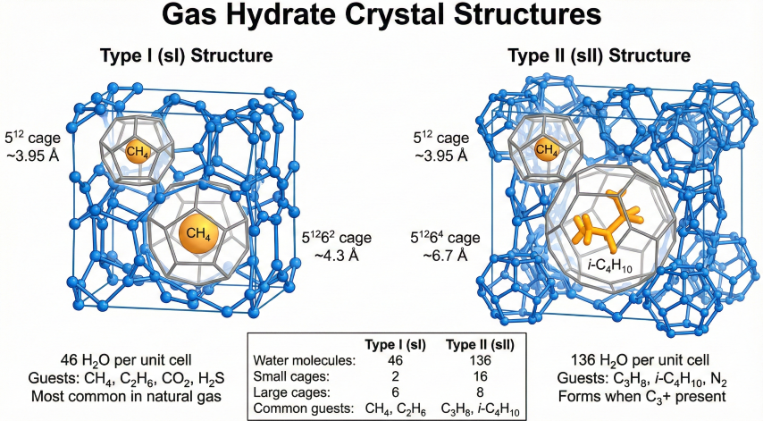
Structure I (sI)
Cavity composition: Two small cages (5¹²) + six large cages (5¹²6²)
Guest molecules: Small gases: CH₄, C₂H₆, CO₂, H₂S
Unit cell: 46 water molecules
Typical in: Natural gas pipelines with primarily methane and ethane
Hydration number: ~6 (one gas molecule per 6 water molecules)
Structure II (sII)
Cavity composition: Sixteen small cages (5¹²) + eight large cages (5¹²6⁴)
Typical in: Rich natural gas with propane and heavier components
Hydration number: ~17 (one gas molecule per 17 water molecules)
Structure H (sH)
Cavity composition: Three small (5¹²), two medium (4³5⁶6³), one large (5¹²6⁸)
Guest molecules: Very large: n-C₅H₁₂, n-C₆H₁₄, methylcyclohexane (requires small helper gas)
Unit cell: 34 water molecules
Typical in: Condensate systems, gas with heavy hydrocarbons
Rare in practice: Less common than sI and sII in field operations
Gas Component
Structure Type
Hydrate Stability
Typical Formation Pressure (at 50°F)
Methane (CH₄)
sI
Moderate
~800 psia
Ethane (C₂H₆)
sI
High
~100 psia
Propane (C₃H₈)
sII
Very high
~30 psia
i-Butane (i-C₄H₁₀)
sII
Very high
~20 psia
n-Butane (n-C₄H₁₀)
sII
High
~25 psia
Carbon dioxide (CO₂)
sI
Very high
~75 psia
Hydrogen sulfide (H₂S)
sI
Very high
~100 psia
Nitrogen (N₂)
sII
Low (requires high P)
>10,000 psia
Thermodynamic Principles
Hydrate formation is governed by thermodynamic equilibrium between the hydrate phase and the gas/liquid water phases:
Hydrate Equilibrium:
Guest Gas (G) + Water (W) ⇌ Hydrate (H)
Chemical potential equilibrium:
μ_H = μ_W + μ_G
Where:
μ = Chemical potential of each phase
Formation conditions (P, T) where all three phases coexist define the hydrate equilibrium curve.
Key principles:
- Higher pressure → Higher hydrate formation temperature
- Richer gas (C₂+, CO₂, H₂S) → Hydrates form more easily (higher T at given P)
- Free water required → No water = no hydrates
- Subcooling → Temperature below hydrate point drives formation rate
Free water (liquid) required for hydrate formation
Water vapor alone insufficient (must condense first)
Sources: Produced water, condensed water vapor, aquifer water
Even small amounts (ppm) can cause blockages over time
4. Gas Composition
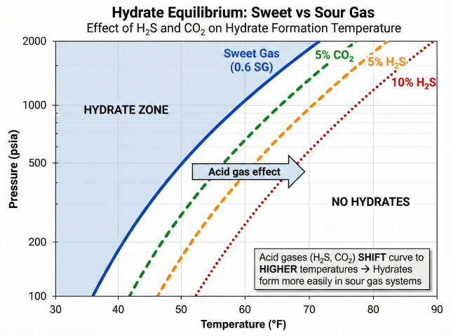
Promoters: C₂H₆, C₃H₈, i-C₄H₁₀, CO₂, H₂S → easier hydrate formation (shift curve right on P-T diagram)
Inhibitors: CH₄ (mild), N₂, heavy HC (C₅+) → harder hydrate formation
Acid gas (CO₂/H₂S) systems form hydrates at much lower pressures than sweet gas
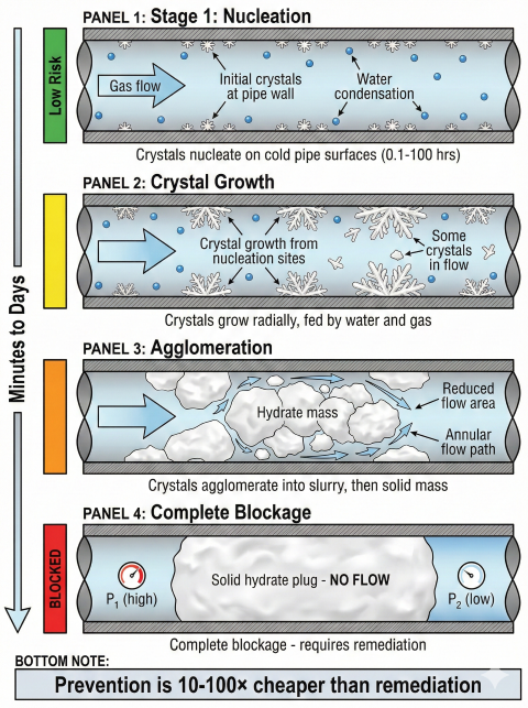
Hydrate Formation Process
Formation Mechanism:
1. Nucleation: Initial crystal formation (rate-limiting step)
- Homogeneous nucleation: Spontaneous in bulk water (slow)
- Heterogeneous nucleation: On surfaces, particles, existing ice (faster)
- Induction time: 0.1–100+ hours (highly variable)
2. Growth: Crystal propagation from nucleation sites
- Radial growth from nucleus
- Controlled by heat and mass transfer
- Faster at higher subcooling
3. Agglomeration: Crystals stick together forming larger masses
- Capillary liquid bridges between particles
- Forms slurries, then plugs
- Most dangerous phase for pipeline blockage
Rate of formation:
dn/dt = k × A × (ΔT_sub)^n × (ΔP)^m
Where:
k = Rate constant (function of gas composition, turbulence)
A = Surface area for growth
ΔT_sub = Subcooling below hydrate point
ΔP = Pressure above minimum hydrate pressure
n, m = Empirical exponents (typically n = 1–2, m = 0.5–1)
Operational risk: Hydrate formation is often unpredictable. Induction time can vary from minutes to days depending on nucleation sites, turbulence, and subcooling. Once nucleation begins, growth and agglomeration can be rapid, leading to plug formation in hours.
2. Prediction Methods
Accurate prediction of hydrate formation conditions is essential for safe pipeline and process design. Methods range from simple empirical correlations to rigorous thermodynamic simulations.
K-Factor (Katz) Method
The Katz K-factor method (1959) is the simplest approach for quick estimates using gravity and pressure.
Katz Gravity Method:
T_hydrate (°F) = A + B × log₁₀(P)
Where:
A, B = Empirical constants based on gas gravity
P = Pressure (psia)
For gas gravity (SG) relative to air:
- SG = 0.6: A = 27.0, B = 16.0
- SG = 0.7: A = 31.0, B = 17.5
- SG = 0.8: A = 35.0, B = 18.5
Example:
SG = 0.6, P = 1000 psia
T_hydrate = 27.0 + 16.0 × log₁₀(1000)
T_hydrate = 27.0 + 16.0 × 3.0 = 75°F
Accuracy: ±5–10°F for sweet natural gas
Limitations: Does not account for acid gases (CO₂, H₂S) or detailed composition
Baillie-Wichert Chart
Graphical method using gas gravity and pressure to read hydrate temperature from chart (GPSA).
Input: Gas specific gravity, pressure (psia)
Output: Hydrate formation temperature (°F)
Accuracy: ±5°F for 0.55 < SG < 0.80, sweet gas
Advantages: Quick reference, no computer needed
Limitations: Sweet gas only, no acid gas correction
Gas Gravity Method with Corrections
Improved Gravity Method (GPSA):
Step 1: Base hydrate temperature from gas gravity
T_base = 27 + 16 × log₁₀(P) [for SG = 0.6 baseline]
Step 2: Correct for actual gas gravity
T_hydrate = T_base + ΔT_SG
Where:
ΔT_SG = 20°F per 0.1 increase in SG above 0.6
(Heavier gas = higher hydrate temperature due to C₂+, C₃+)
Step 3: Acid gas correction (Baillie-Wichert)
T_corrected = T_hydrate + ΔT_acid
Where:
ΔT_acid = +1.0°F per 1 mol% H₂S (strong hydrate promoter)
ΔT_acid = +0.5°F per 1 mol% CO₂ (moderate promoter)
IMPORTANT: H₂S and CO₂ RAISE hydrate formation temperature
(shift equilibrium curve to higher T at same P). This is because
these molecules are excellent "guest" molecules that stabilize the
hydrate cage structure.
Example:
P = 800 psia, SG = 0.7, 5% CO₂
T_base = 27 + 16 × log₁₀(800) = 27 + 16 × 2.903 = 73.4°F
ΔT_SG = (0.7 - 0.6) / 0.1 × 20 = 20°F
ΔT_acid = 5 × 0.5 = 2.5°F
T_hydrate = 73.4 + 20 + 2.5 = 95.9°F
Acid gases (H₂S, CO₂) shift the hydrate curve to higher temperatures - hydrates form more easily in sour gas systems.
Carson-Katz Correlation
More rigorous hand calculation method accounting for detailed gas composition:
Carson-Katz Method:
1. Calculate K-factors for each component:
K_i = y_i / x_i (vapor/liquid equilibrium ratio)
2. Determine hydrate-forming components:
Σ(y_i / K_i) = 1.0 (hydrate equilibrium)
3. Solve iteratively for T at given P using component K-factors
Component K-factors from charts (GPSA) or correlations:
K_CH4, K_C2H6, K_C3H8, K_CO2, K_H2S, etc.
Accuracy: ±3–5°F for natural gas mixtures
Complexity: Requires iteration, component K-factor charts
CSMGem (Colorado School of Mines)
Industry-standard software for rigorous hydrate prediction using statistical thermodynamics:
Method: Van der Waals and Platteeuw statistical thermodynamics model
Inputs: Full gas composition (C1–C5+, CO₂, H₂S, N₂), pressure, temperature
Accuracy: ±1–2°F for well-characterized gas mixtures
Capabilities:
Three-phase equilibrium (vapor-liquid-hydrate)
Inhibitor effect calculations (MeOH, MEG, salts)
Structure prediction (sI, sII, sH)
Inhibitor partitioning in multiphase systems
PVTsim / Multiflash / HYSYS Correlations
Commercial process simulators with built-in hydrate prediction:
Software
Hydrate Model
Accuracy
Best Use Case
PVTsim (Calsep)
Van der Waals-Platteeuw
±1–2°F
PVT analysis, reservoir fluids
Multiflash (KBC)
Infochem model
±1–2°F
Multiphase flow, subsea
HYSYS/UniSim (AspenTech)
Empirical + rigorous
±2–3°F
Process simulation, facilities
OLGA (Schlumberger)
Integrated multiphase
±2–3°F
Dynamic pipeline simulation
PipePhase (Schneider)
Empirical correlations
±3–5°F
Pipeline hydraulics
Typical Hydrate Formation Conditions
Gas Type
Pressure (psia)
Hydrate Temp (°F)
Notes
Dry gas (95% CH₄, 3% C₂H₆)
500
48
Typical pipeline transmission
Dry gas (95% CH₄, 3% C₂H₆)
1000
58
High-pressure transmission
Rich gas (80% CH₄, 10% C₂H₆, 5% C₃H₈)
500
62
Gathering system
Rich gas (80% CH₄, 10% C₂H₆, 5% C₃H₈)
1000
71
Higher risk due to propane
Acid gas (85% CH₄, 10% CO₂)
500
66
CO₂ promotes hydrates
Acid gas (85% CH₄, 10% CO₂)
1000
76
High risk in sour systems
Sour gas (90% CH₄, 5% H₂S)
500
65
H₂S strong promoter
Sour gas (90% CH₄, 5% H₂S)
1000
75
Requires sour service inhibitors
Method selection: Use Katz/gravity methods for screening studies and quick checks. Use CSMGem or equivalent rigorous software for final design, subsea systems, and acid gas applications. Always validate predictions against field experience when available.
Subcooling and Risk Assessment
Subcooling Calculation:
ΔT_sub = T_hydrate - T_actual
Where:
ΔT_sub = Subcooling (°F or °C)
T_hydrate = Predicted hydrate formation temperature at operating pressure
T_actual = Actual fluid temperature
Risk assessment by subcooling:
- ΔT_sub < 5°F: Low risk (margin adequate)
- 5°F ≤ ΔT_sub < 10°F: Moderate risk (monitor, consider inhibitor)
- 10°F ≤ ΔT_sub < 20°F: High risk (inhibitor required)
- ΔT_sub ≥ 20°F: Very high risk (hydrates likely, robust inhibition needed)
Example:
T_hydrate = 65°F at 800 psia (from prediction)
T_actual = 50°F (pipeline flowing temperature)
ΔT_sub = 65 - 50 = 15°F → High risk, inhibitor required
Prediction Accuracy Considerations
Gas composition uncertainty: ±5% composition change can shift T_hydrate by ±3–5°F
Salinity effects: Produced water salinity (NaCl, CaCl₂) depresses hydrate temp by ~1°F per 1 wt% salt
Model limitations: Empirical methods fail for unusual compositions (very rich, very sour)
Safety margin: Design for 10–15°F below predicted hydrate temp to account for uncertainties
3. Inhibition Strategies
Hydrate inhibition prevents or manages hydrate formation through chemical injection, thermal management, or physical removal. Selection depends on economics, operating conditions, and environmental constraints.
Thermodynamic Inhibitors (THI)
Thermodynamic inhibitors shift the hydrate equilibrium curve to lower temperatures (or higher pressures) by reducing water activity.
Methanol (MeOH)
Methanol Properties:
Molecular formula: CH₃OH
Molecular weight: 32.04 g/mol
Freezing point: -143.7°F (-97.6°C)
Boiling point: 148.5°F (64.7°C)
Advantages:
- Highly effective at low concentrations (15–50 wt%)
- Fully miscible with water and gas
- Depresses freezing point and hydrate temp
- Can be injected upstream or at choke
- Regenerable (distillation recovery possible)
Disadvantages:
- Volatile → losses to vapor phase (30–70% to gas)
- Flammable and toxic (requires safety precautions)
- Corrosive to some materials (requires inhibited MeOH)
- High OPEX for high-rate systems
- Environmental concerns (produced water disposal)
Typical dosage: 20–50 wt% in water phase
Depression: ~20–25°F at 30 wt%, ~35–45°F at 50 wt%
Monoethylene Glycol (MEG)
MEG Properties:
Molecular formula: C₂H₆O₂ (HOCH₂CH₂OH)
Molecular weight: 62.07 g/mol
Freezing point: 8.6°F (-13°C)
Boiling point: 387.1°F (197.3°C)
Advantages:
- Low vapor pressure → minimal losses to gas phase (<5%)
- Regenerable via distillation (95–99% recovery typical)
- Less toxic than methanol
- More economical for large systems (lower makeup rates)
- Can be used in closed-loop systems
Disadvantages:
- Requires higher concentrations than MeOH for same depression
- Viscous at low temperatures (flow issues)
- Degrades over time (forms acids, must monitor pH)
- Requires regeneration unit (capital cost)
- Salt and solid buildup in regeneration unit
Typical dosage: 40–80 wt% in water phase
Depression: ~20–25°F at 50 wt%, ~35–45°F at 70 wt%
Regeneration: Vacuum distillation at 250–300°F
Salts (NaCl, CaCl₂)
Salt Inhibition:
Mechanism: Salts dissolved in water reduce water activity (colligative property)
Sodium chloride (NaCl):
- Solubility limit: ~26 wt% at 68°F
- Depression: ~1°F per 1 wt% NaCl
- Maximum depression: ~25–30°F at saturation
Calcium chloride (CaCl₂):
- Solubility limit: ~45 wt% at 68°F
- Depression: ~1.5°F per 1 wt% CaCl₂
- Maximum depression: ~60–70°F at high concentration
Applications:
- Naturally occurring in produced water (partial inhibition)
- Brine injection for hydrate prevention (rare due to scaling)
- Seawater (3.5 wt% NaCl) provides ~3–4°F depression naturally
Limitations:
- Limited depression capability vs. MeOH/MEG
- Scaling and corrosion issues
- Not regenerable
- Density increase affects phase separation
Low-Dosage Hydrate Inhibitors (LDHI)
Low-dosage inhibitors do not prevent hydrate formation thermodynamically but instead modify hydrate crystal growth and agglomeration kinetics.
Kinetic Hydrate Inhibitors (KHI)
KHI Mechanism:
Function: Delay hydrate nucleation and slow crystal growth
Typical chemicals:
- Polyvinylpyrrolidone (PVP)
- Polyvinylcaprolactam (PVCap)
- Anti-freeze proteins (AFP) analogs
Dosage: 0.1–2.0 wt% (based on free water)
Performance:
- Subcooling limit: 10–15°F typical
- Hold time: 6–48 hours before hydrate formation
- Temperature limit: ~50–55°F maximum system temperature
Advantages:
- Very low dosage vs. MeOH/MEG (1–5% of THI volume)
- Lower OPEX and logistics
- Less environmental impact
- No regeneration required
Limitations:
- Limited subcooling capability (not suitable for deepwater)
- Finite hold time (hydrates will eventually form)
- Effectiveness depends on gas composition (poor with CO₂/H₂S)
- Requires rigorous testing for each application
- Not effective if water phase separates (requires turbulence)
Best applications:
- Onshore gas gathering (moderate subcooling)
- Short tie-backs (<20 km)
- Systems with frequent flow (prevents water settling)
Anti-Agglomerants (AA)
AA Mechanism:
Function: Allow hydrates to form but prevent agglomeration into plugs
Typical chemicals:
- Quaternary ammonium compounds
- Alkyl aromatic sulfonates
- Surfactant blends
Dosage: 0.5–3.0 wt% (based on free water)
Performance:
- Allows formation of small, transportable hydrate particles
- Particles remain dispersed in hydrocarbon phase
- Effective at high water cuts (up to 50% water)
Advantages:
- Very low dosage
- No temperature depression limit
- Allows continued flow with hydrates present
- Suitable for high subcooling
Limitations:
- Requires liquid hydrocarbon phase (not for dry gas)
- Water cut must be <50% (particle loading)
- Effectiveness sensitive to surfactant properties
- Difficult to test/qualify (requires flow loops)
- Chemical compatibility with production chemicals
Best applications:
- Oil-dominated systems with free water
- High subcooling environments (deepwater)
- Black oil production
Inhibitor Comparison
Inhibitor Type
Typical Dosage
Depression Capability
CAPEX
OPEX
Best Application
Methanol (MeOH)
20–50 wt% in water
20–50°F
Low
High (losses)
Short-term, small systems, flexible
MEG
40–80 wt% in water
20–50°F
High (regen unit)
Low (recovery)
Large systems, long-term, subsea
KHI
0.5–2.0 wt% in water
10–15°F subcooling
Low
Low
Moderate subcooling, sweet gas
Anti-Agglomerant
0.5–3.0 wt% in water
Unlimited (manages, not prevents)
Low
Low-Medium
Oil systems, high water cut, deepwater
Salts
Natural or injected
~1°F per wt%
Low
Low
Partial credit in produced water
Thermal Methods
Insulation
Pipe-in-pipe (PIP): Annular insulation for subsea pipelines (U-value 0.1–0.3 BTU/hr-ft²-°F)
Wet insulation: Polyurethane or syntactic foam coating
Burial: Onshore pipelines buried below frost line
Effectiveness: Slows cooldown, maintains temp during steady flow; ineffective during shutdown
Heating
Line heaters: Inline heat exchangers (fired or electric)
Heat tracing: Electrical heating cables along pipeline
Hot oil circulation: Jacketed pipe with hot fluid circulation
Direct electrical heating (DEH): Subsea pipelines with electrical current through pipe wall
Application: Maintain temperature above hydrate point during flow or restart
Depressurization
Concept: Reduce pressure to move operating point below hydrate curve
Shutdown procedure: Depressurize pipeline before temperature drops
Limitation: May not be feasible for high-pressure systems or subsea
Strategy selection: Use methanol for small systems, flexibility, or short-term needs. Use MEG for large, long-term systems where regeneration economics are favorable. Use LDHI (KHI or AA) for moderate subcooling and low logistics burden. Always consider combined strategies (insulation + inhibitor) for robust protection.
4. Inhibitor Injection Calculations
Accurate calculation of inhibitor dosage and injection rates is critical for hydrate prevention and cost control.
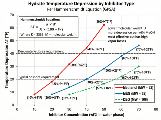
Hammerschmidt Equation (Depression Calculation)
The Hammerschmidt equation (1934) is the industry standard for calculating hydrate temperature depression from thermodynamic inhibitors:
Hammerschmidt Equation (GPSA Equation 20-4):
ΔT = (K × W) / (M × (100 - W))
Where:
ΔT = Hydrate temperature depression (°F)
K = Inhibitor constant = 2335 (°F) for most inhibitors
M = Molecular weight of inhibitor
W = Weight percent inhibitor in aqueous phase (wt%)
Simplified form (K' = K/M pre-calculated):
ΔT = K' × W / (100 - W)
K' Values by Inhibitor:
• Methanol (M=32.04): K' = 2335/32.04 = 72.9
• MEG (M=62.07): K' = 2200/62.07 = 35.4
• DEG (M=106.12): K' = 2222/106.12 = 20.9
Rearranged to solve for required concentration:
W = (100 × ΔT) / (K' + ΔT)
Example (Methanol):
Required depression: ΔT = 20°F
K' = 72.9
W = (100 × 20) / (72.9 + 20)
W = 2000 / 92.9
W = 21.5 wt% methanol in water phase
Example (MEG):
Required depression: ΔT = 25°F
K' = 35.4
W = (100 × 25) / (35.4 + 25)
W = 2500 / 60.4
W = 41.4 wt% MEG in water phase
Valid Range: 10-70 wt% (extrapolation beyond is inaccurate)
Accuracy: ±5% for methanol, ±10% for glycols
Temperature depression by inhibitor type: Lower molecular weight provides more depression per wt%. Methanol most effective but has high vapor losses.
Inhibitor Injection Rate
Inhibitor Injection Rate (Mass Basis):
ṁ_inhibitor = (ṁ_water × W) / (100 - W)
Where:
ṁ_inhibitor = Mass flow rate of inhibitor to inject (lb/hr or kg/hr)
ṁ_water = Mass flow rate of free water in system (lb/hr or kg/hr)
W = Required inhibitor concentration in aqueous phase (wt%)
Example:
ṁ_water = 1,000 lb/hr
W = 30 wt% methanol required
ṁ_MeOH = (1,000 × 30) / (100 - 30)
ṁ_MeOH = 30,000 / 70
ṁ_MeOH = 428.6 lb/hr
Volumetric flow rate:
Q_MeOH = ṁ_MeOH / ρ_MeOH
Where ρ_MeOH = 6.59 lb/gal at 60°F
Q_MeOH = 428.6 / 6.59 = 65 gal/hr
Methanol Loss to Vapor Phase
Methanol is volatile and partitions into the gas phase, requiring additional injection to compensate for losses.
Methanol Vaporization Loss:
Empirical correlation (McCain, 1990):
Loss (lb MeOH/MMscf gas) = 42 × (W / 100) × e^(0.01T - 0.0001P)
Where:
W = MeOH concentration in water (wt%)
T = Temperature (°F)
P = Pressure (psia)
Simplified rule of thumb:
Vapor loss ≈ 30–70% of injected MeOH (higher at low P, high T)
Total MeOH injection:
ṁ_total = ṁ_water_phase / (1 - f_loss)
Where:
f_loss = Fraction lost to vapor (0.3–0.7 typical)
Example:
ṁ_water_phase = 500 lb/hr (MeOH needed for water phase)
f_loss = 0.5 (50% lost to vapor)
ṁ_total = 500 / (1 - 0.5) = 1,000 lb/hr MeOH required
MEG Regeneration Calculation
MEG Regeneration System Sizing:
Rich MEG from separator: 40–60 wt% MEG + water + salts
Lean MEG to injection: 70–90 wt% MEG
Water removal in regeneration unit:
ṁ_water_removed = ṁ_rich_MEG × (W_lean - W_rich) / (100 - W_lean)
Heat duty for regeneration:
Q = ṁ_water_removed × [H_vap + Cp × (T_boiling - T_inlet)]
Where:
H_vap = Latent heat of water (~1,000 BTU/lb at regen conditions)
Cp = Specific heat of water (~1.0 BTU/lb-°F)
T_boiling ≈ 250°F at vacuum conditions in regen unit
Example:
Rich MEG: 50 wt%, 1,000 lb/hr
Lean MEG: 80 wt%
ṁ_water_removed = 1,000 × (80 - 50) / (100 - 80)
ṁ_water_removed = 1,000 × 30 / 20 = 1,500 lb/hr water
Q = 1,500 × [1,000 + 1.0 × (250 - 100)]
Q = 1,500 × [1,000 + 150]
Q = 1,500 × 1,150 = 1,725,000 BTU/hr = 1.725 MMBTU/hr
Reboiler duty for MEG regen: ~1,000–1,500 BTU/lb water removed
Accurate water production rate is essential for inhibitor dosage calculations:
Water Production Rate:
Method 1: Direct measurement
- Test separator water leg
- Multiphase flow meter
Method 2: Water-gas ratio (WGR)
ṁ_water = Q_gas × WGR
Where:
Q_gas = Gas production rate (MMscfd)
WGR = Water-gas ratio (bbl water/MMscf gas), typical 0.1–10 bbl/MMscf
Method 3: Water dewpoint calculation
Water content from gas at saturation (Mcketta-Wehe chart):
w_sat (lb H₂O/MMscf) = f(P, T)
Condensation as gas cools:
ṁ_water = Q_gas × (w_inlet - w_outlet) / 1,000,000
Example:
Q_gas = 50 MMscfd
T_inlet = 120°F, P = 1,000 psia → w_inlet = 150 lb/MMscf
T_outlet = 60°F, P = 1,000 psia → w_outlet = 30 lb/MMscf
ṁ_water = 50 × (150 - 30) / 1,000,000
ṁ_water = 50 × 120 = 6,000 lb/day = 250 lb/hr = 29.9 bbl/day
Safety Margin and Design Philosophy
Inhibitor overdose: Design for 10–25% excess inhibitor to account for:
Water production rate uncertainty (±20% typical)
Injection system turndown limits
Transient upsets (slug flow, well tests)
Model prediction uncertainty (±5°F depression)
Continuous vs. batch injection:
Continuous: Steady-state operation, tight control
Batch: Slug treatment, upstream of long pipelines
Injection point selection:
Upstream of choke (highest risk point for JT cooling)
Wellhead or gathering manifold (earliest protection)
Good mixing essential (atomization nozzle, static mixer)
Field adjustment: Initial inhibitor rates are estimates. Monitor system performance (no hydrate formation, no over-injection waste) and adjust rates based on field data, water production measurements, and downstream analysis of inhibitor concentrations.
Comprehensive Example
Given: Offshore gas pipeline, 20 MMscfd gas, 200 bbl/day water production, P = 1,200 psia, T_hydrate = 68°F, T_flowing = 50°F
Step 1: Determine required depression
ΔT = T_hydrate - T_flowing + margin
ΔT = 68 - 50 + 10 = 28°F (10°F margin for safety)
Step 2: Select inhibitor
Option 1: Methanol (no regeneration, higher OPEX)
Option 2: MEG (regeneration system, lower OPEX)
→ Select MEG for large system (200 bbl/day water)
Step 3: Calculate required MEG concentration (Hammerschmidt)
W = (100 × 62.07 × 28) / (2200 + 62.07 × 28)
W = 173,796 / (2200 + 1,738)
W = 173,796 / 3,938 = 44.1 wt% MEG in water phase
Step 4: Calculate MEG injection rate
ṁ_water = 200 bbl/day × 8.34 lb/gal × 42 gal/bbl = 70,056 lb/day = 2,919 lb/hr
ṁ_MEG = (2,919 × 44.1) / (100 - 44.1)
ṁ_MEG = 128,728 / 55.9 = 2,303 lb/hr
Q_MEG = 2,303 lb/hr / 9.3 lb/gal (MEG density) = 248 gal/hr = 5,950 gal/day = 142 bbl/day
Step 5: Size MEG regeneration system
Rich MEG return: ~45 wt% (diluted by produced water)
Lean MEG target: 75 wt% (sufficient for 28°F depression)
Makeup MEG: ~5–10% of circulation (losses, degradation)
ṁ_makeup = 2,303 × 0.075 = 173 lb/hr = 18.6 gal/hr
Regen unit duty:
Water removal = (45% to 75% reconcentration)
Q_regen ≈ 1.5–2.0 MMBTU/hr reboiler duty
Economics:
MEG cost: $3–5/gal → Makeup ~$450–750/day
Regen fuel: ~50 MMBTU/day × $4/MMBTU = $200/day
Total OPEX: ~$650–950/day + labor + maintenance
Compare to methanol (no regen):
MeOH required: ~150 bbl/day (higher concentration, more losses)
MeOH cost: $5/gal × 6,300 gal/day = $31,500/day
→ MEG regeneration strongly favored for large systems
5. Prevention & Remediation
Design Practices for Hydrate Prevention
Pipeline Design
Insulation: Reduce heat loss, delay cooldown during shutdown
U-value target: <0.3 BTU/hr-ft²-°F for subsea PIP
Cooldown time: Design for 24–72 hours to hydrate conditions
Pig traps and launchers: Allow pigging to remove water accumulation
Low points and traps: Eliminate or provide drainage to prevent water accumulation
Looping: Reduce pressure drop → higher temperature at end of line
Burial depth: Onshore pipelines below frost line (4–6 ft typical)
Process Design
Inlet separation: Remove free water upstream via three-phase separator
Glycol dehydration: Reduce water dewpoint to <7 lb/MMscf (sales gas spec)
Choke placement: Locate downstream of inhibitor injection point
Heating: Maintain temperature above hydrate point via heat exchangers
Depressurization systems: Quick blowdown capability before cooldown
Instrumentation and Monitoring
Temperature monitoring: RTDs at critical points (chokes, low points, subsea)
Pressure monitoring: Track P-T conditions relative to hydrate curve
Flow monitoring: Detect flow restriction from partial plugging
Water analysis: Monitor water cut, inhibitor concentration, salinity
Hydrate prediction software: Real-time calculation of hydrate margin
Operational Procedures
Normal Operations
Inhibitor injection: Continuous injection at calculated rate plus margin
Temperature management: Monitor flowing temperature vs. hydrate temp (maintain 10–15°F margin)
Water removal: Regular separator draining, prevent water buildup
Pigging schedule: Periodic pigging to remove liquids (water, condensate)
Startup Procedures
Pre-startup checks: Verify inhibitor inventory, injection system operational
Inhibitor slug: Inject 2–5× normal rate for first 2–4 hours
Slow ramp: Gradually increase flow to avoid rapid temperature swings
Monitor closely: Temperature, pressure, flow rate during stabilization
Shutdown Procedures
Pre-shutdown inhibitor slug: Increase injection rate 1–2 hours before shutdown
Depressurization: Reduce pressure to below hydrate formation pressure if feasible
Nitrogen blanketing: Displace gas with N₂ (non-hydrate former) for extended shutdown
Drain low points: Remove accumulated water before cooldown
Heat trace activation: Energize electrical heating systems if available
Cold Restart and Hydrate Risk
Restarting a cold, depressurized pipeline presents maximum hydrate risk:
Cold Restart Procedure:
Risk factors:
- Cold pipe (T < hydrate temp at startup pressure)
- Water accumulation during shutdown
- High pressure upon gas introduction
Mitigation steps:
1. Inhibitor pre-treatment: Batch inject MeOH/MEG before introducing gas
2. Low-pressure restart: Start at P < hydrate formation pressure, gradually increase
3. Slow flow ramp: Increase flow slowly to allow warming by gas compression heat
4. Pigging: Pig line to push liquids ahead of gas front
5. Monitoring: Close ΔP surveillance for hydrate plug indications
Example cold restart protocol:
Time 0: Batch inject 50 bbl MeOH into pipeline (slug treatment)
Time +1 hr: Introduce gas at 200 psia (below hydrate pressure)
Time +2 hr: Increase to 400 psia, monitor temperature rise
Time +4 hr: Increase to full operating pressure once T > T_hydrate + 10°F
Time +6 hr: Resume normal inhibitor injection (continuous)
Pressure drop increase: Higher ΔP across pipeline segment
Temperature anomaly: Exothermic hydrate formation → local temperature rise (2–5°F)
Irregular flow: Slugging, instability as hydrates intermittently pass
Indirect Indicators
Subcooling calculation: Real-time T_actual vs. T_hydrate tracking
Trend analysis: Gradual pressure drop increase over hours/days
Inhibitor analysis: Low inhibitor concentration in produced water → insufficient injection
Hydrate Remediation (Plug Removal)
Hydrate plug removal is expensive, time-consuming, and dangerous. Prevention is always preferred.
Hydrate plug formation stages (minutes to days). Prevention is 10-100× cheaper than remediation.
Depressurization Method
Depressurization Procedure:
Concept: Lower pressure to dissociate hydrate (endothermic process)
Steps:
1. Isolate blocked section
2. Slowly depressurize upstream side (avoid rapid Joule-Thomson cooling)
3. Depressurize downstream side simultaneously
4. Monitor pressure equalization (indicates flow through dissociating plug)
5. Continue slow depressurization until fully dissociated
Caution:
- Depressurization is endothermic (ΔH ≈ 50 kJ/mol) → cooling effect
- Rapid depressurization can freeze remaining water → ice blockage
- Gas released from hydrate dissociation (164 volumes CH₄ per volume hydrate at STP)
- Risk of high-velocity gas jet if plug suddenly releases
Depressurization rate: ≤ 100 psi/hr (slow and controlled)
Inhibitor Injection (Soak Method)
Procedure: Inject concentrated methanol (50–100%) at plug location via injection point or wellbore
Soak time: Allow 12–72 hours for methanol to diffuse into hydrate and dissociate
Volume: Large volumes required (100–500 bbl typical) for significant plugs
Circulation: Circulate methanol if possible to enhance contact
Limitation: Slow diffusion into hydrate mass; may take days for large plugs
Heating Methods
Hot oil circulation: Circulate hot oil through annulus or coiled tubing
Electrical heating: Heat tracing or DEH (direct electrical heating) for subsea lines
Hot water injection: Inject hot water (150–180°F) to melt hydrate
Steam injection: High-temperature steam for rapid dissociation (onshore only)
Limitation: Heat transfer limited by insulation, pipe wall; slow for large plugs
Mechanical Methods
Coiled tubing drilling: Drill through hydrate plug (risky, can pack plug tighter)
Pigging: Not effective once plug formed (pig stops at plug)
Line cutting: Last resort for onshore; cut pipe and remove plug mechanically
Remediation costs: Hydrate plug removal costs $100,000–$10,000,000+ depending on location (subsea worst), duration of downtime (lost production), and method used. Prevention via proper inhibition costs 1–10% of remediation cost. Always design for prevention, not remediation.
Safety Considerations
Methanol Handling
Toxicity: Methanol is toxic (LD50 ~100 ml oral); use PPE, ventilation
Flammability: Flash point 52°F; keep away from ignition sources
Corrosion: Use corrosion-inhibited methanol for carbon steel systems
Environmental: Produced water with methanol requires treatment before discharge
Depressurization Hazards
Rapid gas release: Hydrate dissociation releases large volumes of gas suddenly
Cryogenic temperatures: JT cooling during depressurization can cause brittle fracture
Two-phase flow: Liquid slugs during plug dissociation cause pressure surges
Overpressure: Closed systems can overpressure during dissociation (gas expansion)
Subsea Operations
ROV intervention: Limited options for heating, injection, depressurization
Flowline abandonment: Severe plugs may require new flowline (very expensive)