Calculate bottomhole pressure, predict liquid holdup, and analyze gas well performance using Gray's dimensionless number approach. Industry-standard method for high-GLR gas wells per API 14B.
Calculate bottomhole pressure from wellhead conditions
Predict liquid loading onset in gas wells
Size tubing for gas well completions
Evaluate gas lift requirements
1. Overview & Applications
The Gray correlation (1974) is an empirical method for calculating pressure drop in vertical two-phase gas-liquid flow. Developed by H.E. Gray for the API 14B standard on subsurface safety valve sizing, it uses dimensionless groups to correlate liquid holdup with flow conditions.
Primary Use
BHP from Wellhead
Calculate bottomhole flowing pressure given wellhead pressure, flow rates, and fluid properties.
Liquid Loading
Critical Velocity
Determine if gas velocity is sufficient to lift liquids from wellbore (Turner criteria).
Tubing Design
Size Optimization
Balance pressure drop vs. liquid lifting capacity when selecting tubing size.
Gas Lift
Injection Rate
Calculate required gas injection to achieve target bottomhole pressure.
Key Concepts
Two-phase flow: Simultaneous flow of gas and liquid in a conduit; behavior differs from single-phase due to phase interactions
Liquid holdup (HL): Fraction of pipe cross-section occupied by liquid; determines mixture density
Slippage: Gas travels faster than liquid due to buoyancy; causes liquid to accumulate
No-slip holdup (λ): Input liquid fraction if phases traveled at same velocity; λ = Ql/(Ql+Qg)
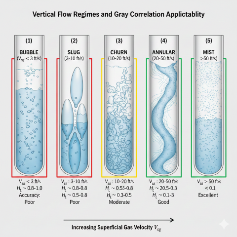
Vertical flow regime progression with Gray correlation applicability ratings for each pattern.
Flow Regime Applicability
Flow Regime
Vsg Range
Characteristics
Gray Accuracy
Bubble
< 3 ft/s
Discrete gas bubbles in liquid
Poor (not designed for this)
Slug
3-10 ft/s
Alternating liquid slugs/gas pockets
Moderate (±20-30%)
Churn
10-20 ft/s
Chaotic oscillating flow
Moderate (±15-25%)
Annular
20-50 ft/s
Liquid film on wall, gas core
Good (±10-15%)
Mist
> 50 ft/s
Liquid droplets in gas
Excellent (±5-10%)
When to use Gray: Vertical or near-vertical wells (<15° deviation) with high GLR (>5,000 scf/bbl) operating in annular or mist flow. For oil wells or high liquid loading, use Hagedorn-Brown instead.
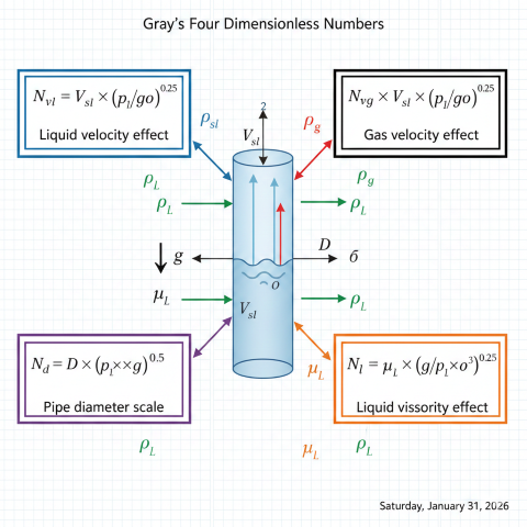
2. Gray Dimensionless Numbers
Gray's correlation uses four dimensionless groups that incorporate fluid properties, pipe geometry, and flow velocities. These numbers normalize the complex physics into universal correlating parameters.
Liquid Velocity Number (Nvl):
Nvl = Vsl × (ρL / (g × σ))0.25
Where:
Vsl = Superficial liquid velocity (ft/s) = Ql / A
ρL = Liquid density (lbm/ft³)
g = Gravitational acceleration (32.17 ft/s²)
σ = Surface tension (lbf/ft) [multiply dyne/cm × 6.85×10⁻⁵]
Gas Velocity Number (Nvg):
Nvg = Vsg × (ρL / (g × σ))0.25
Where:
Vsg = Superficial gas velocity (ft/s) = Qg / A
Qg = Gas volumetric rate at flowing P,T
Pipe Diameter Number (Nd):
Nd = D × (ρL × g / σ)0.5
Where:
D = Pipe inside diameter (ft)
Liquid Viscosity Number (Nl):
Nl = μL × (g / (ρL × σ³))0.25
Where:
μL = Liquid viscosity (lbm/ft·s) [multiply cP × 6.72×10⁻⁴]
Physical Interpretation
Number
Physical Meaning
Typical Range
Nvl
Ratio of liquid inertia to surface tension forces
0.001 - 1.0
Nvg
Ratio of gas inertia to surface tension forces
1 - 500
Nd
Ratio of gravitational to surface tension forces (pipe scale)
50 - 500
Nl
Ratio of viscous to surface tension forces
0.001 - 0.1
Gray dimensionless numbers showing how physical variables combine into correlating parameters.
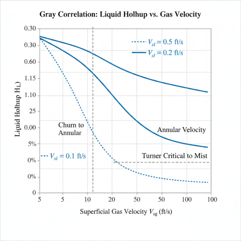
Gray's liquid holdup correlation uses an empirical R-factor to account for slippage between gas and liquid phases. The actual (in-situ) holdup is higher than the no-slip holdup because gas flows faster than liquid.
No-Slip Liquid Holdup:
λ = Vsl / (Vsl + Vsg) = Ql / (Ql + Qg)
This is the holdup if both phases traveled at the same velocity.
Gray R-Factor:
R = (Nvl/Nvg)0.982 × (Nl/Nd)0.124
The R-factor correlates slip behavior with dimensionless numbers.
Psi (ψ) Correlation Factor:
ψ = 1 + R × (R + 0.0814 × ln(R + 0.000925))
This factor amplifies the no-slip holdup to account for slippage.
In-Situ Liquid Holdup:
HL = ψ × λ
Physical limits: 0 < HL ≤ 1.0
Slip Ratio:
S = HL / λ (typically 2-10× for gas wells)
Effect of Holdup on Pressure Drop
Liquid holdup directly affects mixture density, which dominates pressure gradient in vertical wells:
Gray correlation liquid holdup as a function of gas velocity for different liquid loading conditions.
4. Pressure Gradient Calculation
Total pressure gradient in vertical two-phase flow has three components: elevation (hydrostatic head), friction, and acceleration. For most gas well conditions, elevation dominates (80-95% of total).
Total Pressure Gradient:
(dP/dL)total = (dP/dL)elevation + (dP/dL)friction + (dP/dL)accelerationElevation Component (dominant in vertical flow):
(dP/dL)elev = ρm × g × cos(θ) / 144 [psi/ft]
Where:
ρm = Two-phase mixture density (lbm/ft³)
g = 32.17 ft/s²
θ = Deviation from vertical (degrees)
144 = Conversion factor (in²/ft²)
Friction Component:
(dP/dL)fric = f × ρm × Vm² / (2 × gc × D × 144) [psi/ft]
Where:
f = Darcy friction factor (from Colebrook-White)
Vm = Vsl + Vsg (mixture velocity, ft/s)
gc = 32.17 lbm·ft/(lbf·s²)
D = Pipe ID (ft)
Acceleration Component:
Usually negligible for steady-state vertical flow (< 1% of total)
Bottomhole Pressure Calculation
For vertical well (θ = 0°):
PBH = PWH + (dP/dL)total × TVD
Example Calculation:
Given: PWH = 500 psia, TVD = 8,000 ft
ρm = 4.15 lbm/ft³ (from previous example)
f = 0.015, Vm = 56.4 ft/s, D = 0.2034 ft
Elevation gradient:
(dP/dL)elev = 4.15 × 32.17 × 1.0 / 144 = 0.927 psi/ft
Friction gradient:
(dP/dL)fric = 0.015 × 4.15 × 56.4² / (2 × 32.17 × 0.2034 × 144)
(dP/dL)fric = 198 / 1883 = 0.105 psi/ft
Total gradient:
(dP/dL)total = 0.927 + 0.105 = 1.032 psi/ft
Bottomhole pressure:
PBH = 500 + 1.032 × 8,000 = 500 + 8,256 = 8,756 psia
Note: This is a simplified single-segment calculation.
Accurate results require iteration (properties change with depth).
Turner Critical Velocity
The minimum gas velocity to prevent liquid accumulation (loading) in vertical wells:
Gray is one of several empirical correlations for vertical two-phase flow. Selection depends on well type, flow regime, and accuracy requirements.
Correlation Comparison Table
Correlation
Year
Best Application
Limitations
Gray
1974
High GLR gas wells, mist/annular flow
Poor for slug flow, liquid loading
Hagedorn-Brown
1965
Oil wells, high liquid loading, slug flow
Complex charts, less accurate for gas wells
Beggs-Brill
1973
Inclined/horizontal flow, all angles
Developed for horizontal; less accurate for vertical
Duns-Ros
1963
Wide range, flow regime maps
Discontinuities at transitions, complex
Ansari (mechanistic)
1994
All conditions, physics-based
Computationally intensive
When to Use Each Method
Decision Guide:
1. Is it a gas well with GLR > 5,000 scf/bbl?
→ YES: Use Gray (or Duns-Ros)
→ NO: Go to step 2
2. Is liquid loading a concern (low gas rate)?
→ YES: Use Hagedorn-Brown or Ansari mechanistic
→ NO: Go to step 3
3. Is deviation > 15° from vertical?
→ YES: Use Beggs-Brill
→ NO: Gray or Hagedorn-Brown acceptable
4. Is high accuracy required (±5%)?
→ YES: Use mechanistic model (Ansari, Hasan-Kabir)
→ NO: Gray is acceptable for screening
Industry Practice:
Run multiple correlations and compare. If results differ by >20%,
investigate flow regime and validate with field pressure surveys.
Accuracy Comparison (Field Studies)
Well Type
Gray Error
Hagedorn-Brown Error
Recommended
High-rate gas (>5 MMscfd)
±8%
±15%
Gray
Low-rate gas with loading
±25%
±12%
Hagedorn-Brown
Gas condensate (20-50 bbl/MMscf)
±12%
±10%
Either acceptable
Oil well (GOR > 1,000)
±18%
±9%
Hagedorn-Brown
Summary: Gray correlation is the industry standard for vertical gas wells with high GLR operating in annular or mist flow. For oil wells, high liquid loading, or slug flow conditions, Hagedorn-Brown provides better accuracy. Always validate predictions with measured bottomhole pressure when available.