Calculate flare header backpressure using API 521 guidelines, evaluate relief valve capacity effects, and perform network hydraulic analysis for safe pressure relief system design.
Verify flare header backpressure compliance with API 521.
Size flare headers for multiple relief scenarios.
Select appropriate relief valve type (conventional vs balanced).
1. Overview & API 521 Criteria
Flare backpressure is the pressure at the outlet of a pressure relief valve (PRV) caused by flow resistance in the downstream flare system. Excessive backpressure reduces PRV capacity and can prevent proper overpressure protection.
Built-up backpressure
Dynamic pressure
Pressure increase during relief event due to flow through header and stack.
Superimposed backpressure
Static pressure
Constant pressure at PRV outlet before relief (atmospheric + liquid seal).
Total backpressure
Built-up + Superimposed
Sum of static and dynamic components during relief event.
Critical parameter
Affects PRV capacity
High backpressure reduces effective PRV discharge capacity significantly.
Key Concepts
Set pressure: Gauge pressure at which PRV begins to open (psig)
Overpressure: Pressure increase above set pressure, typically 10% or 21% (ASME limits)
Built-up backpressure: Pressure rise in discharge system during flow
Conventional PRV: Spring-loaded valve with bonnet vented to atmosphere
Balanced PRV: Bellows or pilot-operated valve compensating for backpressure
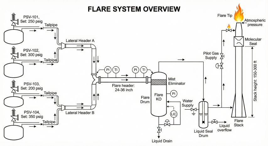
Typical flare system showing backpressure development from PRV to atmosphere.
Why backpressure matters: A conventional PRV at 100 psig set pressure with 15 psig backpressure (15% of set) violates API 521 limits and loses approximately 30% of its rated capacity. This can result in inadequate overpressure protection.
API 521 Design Philosophy
API Standard 521, "Pressure-relieving and Depressuring Systems," provides industry-accepted guidelines for flare system design. Key principles include:
Backpressure limits ensure PRV operates as designed per ASME Section VIII
Multiple concurrent relief scenarios must be evaluated (not just single largest)
Dynamic simulation recommended for complex networks with time-varying flows
Flare tip design must handle maximum credible discharge without excessive noise or radiation
2. Header Pressure Drop
Pressure drop in flare headers is the primary component of built-up backpressure. Accurate calculation requires consideration of gas properties, flow regime, and system geometry.
Darcy-Weisbach Equation
Incompressible Flow (ΔP/P < 10%):
ΔP = f × (L/D) × (ρ V²/2)
Where:
ΔP = Pressure drop (psf or Pa)
f = Darcy friction factor (dimensionless)
L = Pipe length (ft or m)
D = Inside diameter (ft or m)
ρ = Gas density (lb/ft³ or kg/m³)
V = Gas velocity (ft/s or m/s)
Converting to common units:
ΔP (psi) = f × (L/D) × (ρ V²) / (2 × 144)
For V in ft/s, ρ in lb/ft³
Friction Factor Calculation
Reynolds Number:
Re = ρ V D / μ
Where:
μ = Dynamic viscosity (lb/ft·s or Pa·s)
Friction Factor (Colebrook-White):
For turbulent flow (Re > 4000):
1/√f = -2 log₁₀[(ε/D)/3.7 + 2.51/(Re √f)]
Where:
ε = Absolute pipe roughness (ft or m)
ε/D = Relative roughness
Typical ε values:
- Commercial steel: 0.00015 ft (0.046 mm)
- Stainless steel: 0.000007 ft (0.002 mm)
- Corroded steel: 0.0010 ft (0.30 mm)
Solved iteratively or use Moody diagram.
Compressible Flow Correction
For significant pressure drop (ΔP/P > 10%), compressibility effects must be included:
Isothermal Compressible Flow:
P₁² - P₂² = (f × L × ρ₁ × V₁² × P₁) / D
Or using mass flux:
P₁² - P₂² = (f × L × G² × R × T × Z) / (D × MW)
Where:
G = Mass flux (lb/ft²·s or kg/m²·s)
R = Universal gas constant
T = Absolute temperature (°R or K)
Z = Compressibility factor
MW = Molecular weight
For typical flare gas (MW ≈ 25, Z ≈ 1.0):
Solve for P₂ iteratively given inlet P₁, flow rate, and geometry.
Fittings and Valves
Pressure drop through elbows, tees, and valves adds to straight pipe losses:
Equivalent Length Method:
L_total = L_straight + Σ(K × D / f)
Where:
K = Resistance coefficient for each fitting
Common K values:
- 90° elbow: K = 30 (long radius), 60 (short radius)
- 45° elbow: K = 16
- Tee (flow through): K = 20
- Tee (flow branch): K = 60
- Gate valve (open): K = 8
- Check valve: K = 100
Alternatively, direct loss coefficient:
ΔP_fitting = K × (ρ V² / 2)
Two-Phase Flow Considerations
Flow Regime
Characteristics
Pressure Drop Impact
All vapor
Dry gas relief
Use gas correlations above
Mist flow
< 5% liquid by volume
Use homogeneous model, +10-20% safety factor
Annular/slug
5-30% liquid volume
Use Lockhart-Martinelli or Friedel correlation
Churn/bubble
> 30% liquid volume
Liquid-dominant: use liquid friction factor + holdup
Example Calculation
Calculate pressure drop in 500 ft of 12-inch schedule 40 flare header (ID = 11.938 in = 0.995 ft) carrying 50,000 lb/hr of natural gas at 30 psia and 100°F:
Given:
W = 50,000 lb/hr = 13.89 lb/s
D = 0.995 ft
A = π D²/4 = 0.778 ft²
P = 30 psia
T = 100 + 460 = 560 °R
SG = 0.60, MW = 0.60 × 28.97 = 17.4 lb/lbmol
μ = 0.011 cP = 7.4 × 10⁻⁶ lb/ft·s
Z ≈ 1.0
ρ = (P × MW) / (Z × R × T)
ρ = (30 × 17.4) / (1.0 × 10.73 × 560) = 0.087 lb/ft³
V = W / (ρ × A) = 13.89 / (0.087 × 0.778) = 205 ft/s
Re = ρ V D / μ = (0.087 × 205 × 0.995) / (7.4 × 10⁻⁶)
Re = 2.41 × 10⁶ (highly turbulent)
For ε = 0.00015 ft (commercial steel):
ε/D = 0.00015 / 0.995 = 0.000151
Using Colebrook-White (or Moody chart):
f ≈ 0.0145
ΔP = f × (L/D) × (ρ V²) / (2 × 144)
ΔP = 0.0145 × (500/0.995) × (0.087 × 205²) / (2 × 144)
ΔP = 0.0145 × 503 × 3657 / 288
ΔP = 92.5 psi
This is significant compression (ΔP/P = 92.5/30 = 308%), so incompressible
assumption invalid. Must use compressible flow equations.
Using isothermal compressible:
P₁² - P₂² = (f × L × W² × R × T × Z) / (D⁵ × ρ₁ × π²)
Solving iteratively: P₂ ≈ 28.2 psia
Built-up backpressure ΔP = 30 - 28.2 = 1.8 psi ✓
Note: High velocity (205 ft/s) causes this pressure drop. API 521 recommends
header velocity < 0.5 Mach (~600 ft/s for gas) to avoid excessive pressure drop.
3. Backpressure Limits per API 521
API Standard 521 and ASME Section VIII establish maximum allowable backpressure based on relief valve type to ensure proper operation and rated capacity.
Conventional Spring-Loaded PRVs
API 521 Conventional PRV Limits:
Built-up backpressure ≤ 10% of set pressure
For set pressure = 100 psig:
Maximum built-up BP = 10 psig
Superimposed backpressure ≤ 10% of set pressure (additional limit)
Total backpressure = Superimposed + Built-up ≤ 10% + 10% = 20%
Rationale:
Conventional PRVs vent bonnet to atmosphere. Backpressure on discharge
side creates upward force on disc reducing net opening force. Exceeding
10% causes:
- Reduced capacity (can lose 30-50% at 15% BP)
- Chattering and instability
- Premature seat wear
Balanced Bellows PRVs
API 521 Balanced PRV Limits:
Built-up backpressure ≤ 50% of set pressure
For set pressure = 100 psig:
Maximum built-up BP = 50 psig
Superimposed backpressure ≤ 10% of set pressure
Total backpressure ≤ 50% (built-up) + 10% (superimposed) = 60%
Mechanism:
Bellows isolates bonnet from discharge pressure, compensating for
backpressure effects. Allows much higher BP before capacity loss.
Limitations:
- Bellows can rupture (requires monitoring)
- More expensive than conventional
- Capacity correction factor still applies (K_b < 1.0)
Pilot-Operated PRVs
Pilot-Operated Valve Limits:
Built-up backpressure: Manufacturer specific, often up to 90% of set
Superimposed backpressure ≤ 50% of set pressure
Advantages:
- Excellent for high backpressure applications
- Tight shutoff (no simmer)
- Large turndown ratio
Disadvantages:
- Requires clean service (pilot can clog)
- More complex than spring-loaded
- May require instrument air supply
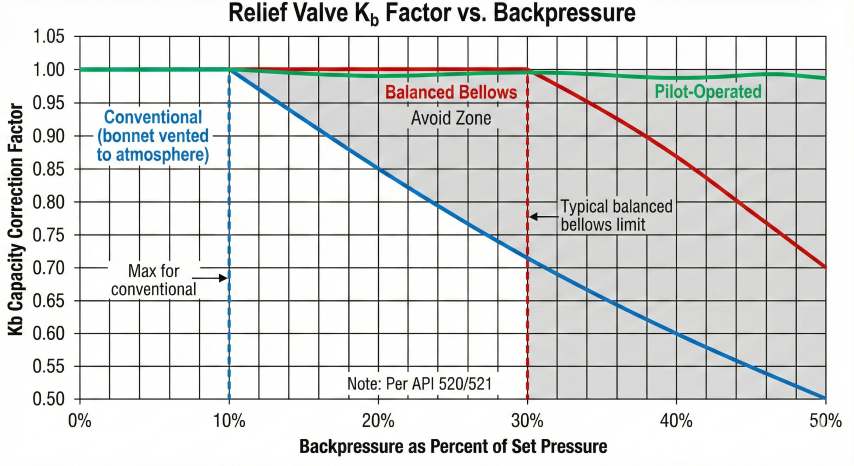
Capacity Correction Factors
Backpressure correction factor (Kb) curves per API 520 Figures 30 & 31.
Valve Type
Backpressure Correction
Typical K_b Range
Source
Conventional
Required for BP > 0%
0.50–1.00
API 520 Fig. 30
Balanced bellows
Required for BP > 30%
0.70–1.00
API 520 Fig. 31
Pilot-operated
Minimal correction
0.90–1.00
Manufacturer data
Calculating Required Orifice Area with Backpressure
ASME Section VIII Gas Relief (API 520 Form):
A = (W / (C × K_d × P₁ × K_b)) × √(T × Z / M)
Where:
A = Required orifice area (in²)
W = Required flow capacity (lb/hr)
C = Coefficient (315 for gas with K = 1.4)
K_d = Discharge coefficient (typically 0.975)
P₁ = Upstream relieving pressure (psia)
= Set pressure × (1 + overpressure) + atmospheric
K_b = Backpressure correction factor (< 1.0)
T = Relieving temperature (°R)
Z = Compressibility factor at relieving conditions
M = Molecular weight
Example with backpressure penalty:
W = 50,000 lb/hr natural gas
Set = 100 psig (114.7 psia)
Overpressure = 10% (code max for fire case)
P₁ = 114.7 × 1.10 = 126.2 psia
T = 560 °R, Z = 1.0, M = 17.4
K_d = 0.975
Case 1: No backpressure (K_b = 1.0)
A = (50,000 / (315 × 0.975 × 126.2 × 1.0)) × √(560 × 1.0 / 17.4)
A = (50,000 / 38,737) × 5.67 = 7.31 in²
Select ASME orifice P (11.05 in²) - provides margin
Case 2: With 12 psig backpressure (12% of set)
Conventional valve: EXCEEDS 10% limit → cannot use conventional
Balanced valve: OK, but K_b ≈ 0.92 per vendor curve
A = (50,000 / (315 × 0.975 × 126.2 × 0.92)) × √(560 × 1.0 / 17.4)
A = (50,000 / 35,638) × 5.67 = 7.95 in²
Still fits orifice P, but with less margin.
Backpressure increased required area by 9%.
Economic impact: Exceeding backpressure limits requires upgrading to balanced or pilot-operated valves (2-3× cost), or increasing flare header diameter (very expensive retrofit). Proper sizing at design stage is critical.
4. Multiple Relief Sources & Accumulation
Flare headers collect relief from multiple PRVs across a facility. Simultaneous relief scenarios must be evaluated to ensure backpressure limits are met during credible concurrent events.
Relief Scenario Development
API 521 requires evaluation of multiple relief scenarios, not just the single largest source:
Single largest source: Individual PRV at maximum capacity (e.g., compressor discharge PSV)
Fire case: All equipment in a fire zone relieving simultaneously per API 521 Annex C
Power failure: Loss of cooling causes multiple vessels to relieve
Blocked outlet: Downstream isolation causes multiple PRVs to open
Process upset: Tower flooding, heat exchanger tube rupture, etc.
Fire Relief Accumulation (API 521 Annex C)
Fire Relief Flow Rate:
Q = 21,000 × F × A^0.82
Where:
Q = Required relief rate (lb/hr)
F = Environment factor (1.0 for good drainage/firefighting)
A = Total wetted surface area exposed to fire (ft²)
Wetted Area (vertical vessel):
A_w = π × D × L_wetted
Where:
D = Vessel diameter (ft)
L_wetted = Height from bottom to normal liquid level (ft)
For a 10 ft diameter × 30 ft tall vessel, 50% liquid:
A_w = π × 10 × 15 = 471 ft²
Q = 21,000 × 1.0 × 471^0.82 = 21,000 × 119 = 2.5 million lb/hr
If five such vessels are in one fire zone:
Total Q = 5 × 2.5 = 12.5 million lb/hr to common header
This enormous flow requires large header (36-48 inch) to keep ΔP < 10%.
Staggered Relief (Credit for Time Delays)
Some scenarios allow credit for time-staggered relief if physical delays are demonstrated:
Vessel Heatup Time to Relief:
t = (m × Cp × ΔT) / Q_fire
Where:
t = Time to reach set pressure (minutes)
m = Liquid inventory mass (lb)
Cp = Specific heat (Btu/lb·°F)
ΔT = Temperature rise from normal to relief (°F)
Q_fire = Fire heat input rate (Btu/hr)
If two vessels have heatup times of 10 min and 25 min respectively,
peak relief may not be simultaneous. Dynamic simulation can capture this.
Warning: API 521 discourages taking credit for staggered relief
without rigorous thermal/hydraulic modeling due to uncertainty in fire exposure.
Header Segment Approach
Complex flare networks are divided into segments, each analyzed for worst-case backpressure:
Header Segment
Contributing Sources
Design Scenario
Peak Flow (lb/hr)
Compressor Area
3× compressor PSVs
Power failure
75,000
Storage Area
5× tank PRVs
Fire case
120,000
Process Area
10× vessel PSVs
Blocked outlet
200,000
Main Header
All above
Site-wide fire
395,000
Probability-Based Design
Modern practice sometimes uses risk-based design for extremely low-probability concurrent events:
Deterministic approach (traditional): Size for worst credible case, all fire zones simultaneously
Risk-based approach: Use frequency analysis to determine acceptance of minor exceedances during 1-in-1000-year events
API 521 position: Conservative deterministic approach required unless risk assessment formally approved by owner/regulator
Design conservatism: Most facilities size flare headers for "all equipment in largest fire zone relieving simultaneously" as base case, then verify no credible scenario exceeds this. This provides substantial safety margin against uncertainties.
5. Network Hydraulic Analysis
Complex flare systems with multiple headers, knockout drums, and parallel paths require network hydraulic modeling to accurately predict backpressure at each relief valve.
Network Components
Flare header
Main collection piping
Primary pressure drop component; typically 12-48 inch carbon steel.
Knockout drum
Liquid separation
Removes entrained liquids before flare tip; introduces pressure drop.
Flare stack
Vertical riser to tip
Elevation head and friction; 100-300 ft tall typical.
Molecular seal/purge
Flame arrestor
Prevents flashback; adds resistance but essential for safety.
Hardy Cross Method (Manual Network Balancing)
For simple networks, the Hardy Cross iterative method can solve for flows and pressures:
Hardy Cross Loop Equations:
For each loop in the network, conservation of pressure drop:
Σ ΔP_loop = 0
For each node, conservation of mass:
Σ W_in = Σ W_out
Iteration procedure:
1. Assume initial flow distribution in each pipe segment
2. Calculate ΔP for each segment using Darcy-Weisbach
3. For each loop, compute Σ ΔP (should be zero if balanced)
4. Adjust flows using correction factor:
ΔW = -Σ(ΔP) / Σ(ΔP/W)
5. Repeat until Σ ΔP < tolerance (e.g., 0.1 psi)
Converges in 3-5 iterations for typical flare networks.
Computational Network Modeling
Modern practice uses specialized software for flare network analysis:
Aspen HYSYS Flare: Dynamic simulation with time-varying relief, integrated with process model
Aspen Flare System Analyzer: Steady-state and dynamic flare network sizing
PIPENET: General pipe network solver adaptable to flare systems
For complex scenarios with time-varying flows, dynamic simulation captures pressure wave propagation:
Transient Flow Equations:
Continuity:
∂ρ/∂t + ∂(ρV)/∂x = 0
Momentum:
∂V/∂t + V ∂V/∂x = -(1/ρ) ∂P/∂x - (f V² / 2D) - g sin(θ)
Solved using method of characteristics or finite difference.
Applications:
- Pressure surge when large PRV opens suddenly
- Relief valve instability (chattering)
- Flare tip blowout risk during rapid gas influx
- Liquid carryover into flare stack
Dynamic models predict peak transient BP may exceed steady-state by 20-50%.
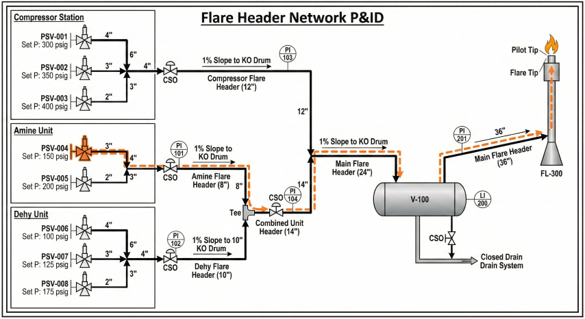
Multi-source flare network with pressure drop calculation points.
Example Network Problem
Consider a simplified flare network with two relief sources joining a common header:
Given:
Source A: 30,000 lb/hr through 150 ft of 8-inch pipe
Source B: 50,000 lb/hr through 200 ft of 10-inch pipe
Both join 12-inch main header (500 ft to KO drum)
Gas properties: MW = 20, SG = 0.69, T = 100°F
Header pressure at KO drum = 5 psig (19.7 psia)
Find backpressure at Source A and Source B outlets.
Step 1: Calculate pressure drop in 12-inch main header (total flow)
W_total = 30,000 + 50,000 = 80,000 lb/hr
(Use Darcy-Weisbach with f ≈ 0.015, D = 0.995 ft)
Result: ΔP_main ≈ 3.2 psi
Junction pressure = 19.7 + 3.2 = 22.9 psia
Step 2: Calculate ΔP in 8-inch lateral (Source A)
W = 30,000 lb/hr, L = 150 ft, D = 7.981 in = 0.665 ft
Result: ΔP_A ≈ 2.8 psi
Backpressure at A = 22.9 + 2.8 = 25.7 psia = 11.0 psig
Step 3: Calculate ΔP in 10-inch lateral (Source B)
W = 50,000 lb/hr, L = 200 ft, D = 10.02 in = 0.835 ft
Result: ΔP_B ≈ 2.1 psi
Backpressure at B = 22.9 + 2.1 = 25.0 psia = 10.3 psig
Conclusion:
If both PRVs have set pressure 100 psig:
Source A: BP = 11.0% of set → EXCEEDS 10% conventional limit
Source B: BP = 10.3% of set → EXCEEDS 10% conventional limit
Both require balanced bellows or pilot-operated valves, or increase header size.
Design Optimization Strategies
Strategy
Implementation
Typical Cost
Effectiveness
Increase header diameter
Upsize from 12" to 16"
$$$
ΔP reduced by ~60% (∝ D⁵)
Reduce header length
Relocate flare stack closer
$$$$
ΔP ∝ L (linear reduction)
Use balanced PRVs
Replace conventional valves
$
Allows 50% BP vs 10%
Pilot-operated PRVs
For high BP locations
$$
Allows up to 90% BP
Multiple flare systems
Separate HP/LP flares
$$$$$
Eliminates mixing issues
Add intermediate KO
Pressure break in network
$$$
Segments system hydraulically
Best practice: Size flare headers for 10% or less backpressure using conventional PRVs as baseline. This maximizes relief valve options, simplifies maintenance (conventional valves are more robust), and provides margin for future plant expansions without header modifications.
Common Pitfalls
Ignoring fittings and valves: A header with 20 elbows can have 30% more pressure drop than straight pipe calculation suggests
Using incompressible equations for high ΔP/P: Compressibility correction required when ΔP > 10% of inlet pressure
Neglecting elevation head: 100 ft stack height adds ρgh pressure drop (0.5-1.0 psi for typical gas density)
Assuming steady-state flow: Transient pressure spikes can exceed steady-state by 20-50% when large PRVs open rapidly
Not accounting for future expansions: Flare header retrofits are extremely expensive; oversizing 20-30% at design stage is prudent